
EIGEN DECOMPOSITION
- Aryan

- Mar 23, 2025
- 4 min read
SOME SPECIAL MATRICES
Diagonal Matrix
A diagonal matrix is a type of square matrix where the entries outside the main diagonal are all zero; the main diagonal is from the top left to the bottom right of the square matrix.
a. Powers: The nth power of a diagonal matrix (where n is a non-negative integer) can be obtained by raising each diagonal element to the power of n.
b. Eigenvalues: The eigenvalues of a diagonal matrix are just the values on the diagonal. The corresponding eigenvectors are the standard basis vectors.
c. Multiplication by a Vector: When a diagonal matrix multiplies a vector, it scales each component of the vector by the corresponding element on the diagonal.
d. Matrix Multiplication: The product of two diagonal matrices is just the diagonal matrix with the corresponding elements on the diagonals multiplied.
Orthogonal Matrix
An orthogonal matrix is a square matrix whose columns and rows are orthogonal unit vectors (i.e., orthonormal vectors), meaning that they are all of unit length and are at right angles to each other.
Perfect rotation, no scaling or shearing.
a. Inverse Equals Transpose: The transpose of an orthogonal matrix equals its inverse, i.e., 𝐴ᵀ = 𝐴⁻¹. This property makes calculations with orthogonal matrices computationally efficient.
Symmetric Matrix
A symmetric matrix is a type of square matrix that is equal to its own transpose. In other words, if you swap its rows with columns, you get the same matrix.
a. Real Eigenvalues: The eigenvalues of a real symmetric matrix are always real, not complex.
b. Orthogonal Eigenvectors: For a real symmetric matrix, the eigenvectors corresponding to different eigenvalues are always orthogonal to each other. If the eigenvalues are distinct, you can even choose an orthonormal basis of eigenvectors.
MATRIX COMPOSITION
When we multiply the matrices

the product of this multiplication is also a matrix.
The geometric intuition behind this is as follows: When we apply the transformation represented by

to a vector, it transforms the vector. Then, when we apply the transformation

to the already transformed vector, the vector undergoes another transformation. Instead of applying these two transformations separately, we can combine them into a single transformation :

which represents the result of multiplying the two matrices .

MATRIX DECOMPOSITION
Matrix decomposition is the reverse process of matrix composition. Suppose we have a matrix D, and we break it down into matrices A , B , and C.
When we multiply A , B , and C together, we obtain matrix D. This process is called composition.
When we break matrix D into simpler matrices like A , B , and C , this is called matrix decomposition.
Matrix decomposition is useful in many mathematical and computational applications, as it simplifies complex matrix operations into more manageable parts .
EIGEN DECOMPOSITION
The eigen decomposition of a matrix A is given by the equation:
A = VΛ𝑉⁻¹
Where:
V is a matrix whose columns are the eigenvectors of A
Λ is a diagonal matrix whose entries are the eigenvalues of A
𝑉⁻¹ is the inverse of V
Assuming
Square matrix : Eigen decomposition is only defined for square matrices
Diagonalizability : For a n*n matrix it should have n linearly independent eigen vectors.
Suppose we have a matrix A given by :
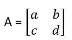
It has eigenvalues λ1 and λ2 , and the corresponding eigenvectors :
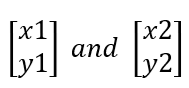
Using these, we can express A as :
A = VΛ𝑉⁻¹
Where :

In simpler terms, this means we can decompose the matrix A into the product of three matrices: P, D, and 𝑃⁻¹. This process is known as eigen decomposition .
EIGEN DECOMPOSITION OF SYMMETRIC MATRIX
Consider a symmetric matrix A :

The equation A = VΛ𝑉⁻¹ holds, but for symmetric matrices, this is specifically called spectral decomposition rather than eigen decomposition. Since A is symmetric, we refer to this process as spectral decomposition.
Key Properties
V is an orthogonal matrix, meaning its columns are orthonormal eigenvectors of A.
Λ is a diagonal matrix whose diagonal elements are the eigenvalues of A.
Thus, we can decompose the symmetric matrix A as:
A=VΛ𝑉⁻¹
Since V is orthogonal, it represents a rotation transformation. The diagonal matrix Λ performs scaling, and because V⁻¹ is also orthogonal, it applies another rotation transformation .
Interpretation
The linear transformation corresponding to a symmetric matrix consists of three operations: rotation → scaling → rotation. This decomposition provides a fundamental understanding of how symmetric matrices transform vectors in space.
How PCA Utilizes Eigen decomposition
Principal Component Analysis (PCA) is a technique that transforms a dataset into a new coordinate system, capturing the most significant variance along principal axes. This transformation is achieved through eigen decomposition of the covariance matrix.
Steps in PCA Using Eigen decomposition :
Centering the Data:
The mean of each predictor variable is subtracted from the dataset to center it around zero.
Constructing the Covariance Matrix:
The covariance matrix is an n * n symmetric matrix that describes how different features vary together.
The diagonal elements represent the variance of each feature, while off-diagonal elements indicate the covariance between different features.
Applying Eigen decomposition:
The covariance matrix is decomposed into eigenvectors and eigenvalues.
Eigenvectors define new axes (principal components) along which variance is maximized.
Eigenvalues indicate the amount of variance explained by each principal component.
Transforming the Data:
The original dataset is projected onto the eigenvectors, effectively rotating and scaling it.
This transformation results in new feature representations that capture the most important variations in the data.
Why PCA Uses Eigen decomposition ?
Identifies relationships between features using the covariance matrix.
Determines the directions of maximum variance using eigenvectors.
Ranks these directions based on importance using eigenvalues.
Reduces dimensionality while preserving significant patterns in the data.
In essence, PCA rotates, scales, and transforms the dataset to align it along principal components, ensuring the best variance representation on specific axes.


