LOGISTIC REGRESSION - 3

Understanding Probability and Likelihood through Examples

Example 1 : Coin Toss (Bernoulli Distribution)

Let’s begin with a simple random experiment : flipping a coin.

Suppose we are given a fair coin, which means it has two equally likely outcomes :

• Head (H)

• Tail (T)

We are told that the probability of getting a head is 0.5

Now, what is the probability of getting tail in one flip ?

Since the coin is fair, the answer is straightforward :

P(T) = 1−P(H) = 1−0.5 = 0.5

We can also model this situation using a Bernoulli distribution, which is used to model experiments with only two outcomes (success/failure, yes/no, head/tail).

The Bernoulli distribution has one parameter :

• p : probability of success (in our case, getting a head)

• q = 1−p : probability of failure (getting a tail)

The probability mass function (PMF) of the Bernoulli distribution is :

• If k = 1 , we are finding the probability of head → P(X = 1) = p

• If k=0 , we are finding the probability of tail → P(X = 0) = 1−p

So, using this function, we can determine the probability of an outcome based on a known parameter p.

This process—using known parameters to compute the chance of an event—is what we call probability.

Definition of Probability :

Given a known distribution and known parameters, probability measures the chance of observing a particular event.

What is Likelihood ?

Now let’s look at the same experiment from a different perspective.

Suppose you flipped a coin 5 times and observed 5 heads in a row.

You begin to wonder : Is the coin really fair ?

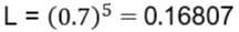
If the coin were truly fair, then the probability of getting 5 heads in a row would be :

This value is very small, which raises doubt about whether the coin is actually fair.

This is the essence of likelihood.

In this case :

• The data is fixed : 5 heads

• The parameter (p) is uncertain

• We evaluate how likely it is that the observed data came from a distribution where p = 0.5

This is likelihood.

Definition of Likelihood :

Given observed data, likelihood measures how plausible a particular value of the model parameter is.

We can also try other values of p . Suppose we consider a biased coin where :

p = 0.7(probability of head)

Then the likelihood becomes :

Now compare :

This means :

Observing 5 heads is more likely if the coin has p = 0.7 than if it had p = 0.5

This demonstrates how likelihood helps us evaluate different parameter values based on the data we observe.

• When you know the parameter, and you want to compute the chance of some event → this is probability.

• When you observe the event, and you want to assess how well a parameter explains it → this is likelihood.

Both concepts are deeply connected, but the direction of inference is reversed.

Example 2 : Drawing Balls from a Bag

Let’s consider a bag that contains :

• 3 red balls

• 2 green balls

This is a closed bag, and we are randomly drawing one ball at a time. Based on this setup, the probability of drawing a green ball is :

What kind of distribution does this random experiment follow ?

Since we are drawing one ball and there are only two possible outcomes (Red or Green), this experiment follows a Bernoulli distribution.

In the Bernoulli distribution :

• Let success be defined as drawing a green ball.

• Then, the parameter p (probability of success) is :

• Accordingly, the probability of failure (drawing a red ball) is :

The probability mass function (PMF) is again :

Let’s say we want to compute the probability of drawing a red ball :

• Let k = 0 (representing red)

• Then :

So, we have:

• Known distribution : Bernoulli

• Known parameter :

• Question: What is the chance of drawing a red ball ?

This is a classic use of probability, because :

We know the parameter, and we are calculating the chance of an event.

Now, Let’s Understand Likelihood

Suppose we perform this experiment 5 times and observe the following outcome:

All 5 draws result in green balls

This raises a natural question :

Is it still reasonable to believe that the probability of green is only 2/5 ?

Let’s calculate the likelihood of seeing 5 green balls, assuming p = 2/5 :

This is a very small number, indicating that :

• It is highly unlikely to observe 5 green balls in a row if the probability of green is truly 2/5

Now, suppose instead the bag had :

• 4 green balls

• 1 red ball

Then, p = 4/5 . Let’s compute the likelihood under this assumption :

Compare the two likelihoods :

This tells us :

• Observing 5 green balls is more likely if the bag has a higher proportion of green balls

• Therefore, the likelihood that p = 4/5 is greater than the likelihood that p =  2/5

• If we know the parameter and ask about an event → this is probability.

• If we observe an event and ask about the parameter → this is likelihood.

Both are built on the same mathematical foundation but serve different purposes in statistical reasoning.

Example 3 : Normal Distribution – Height of a Person

Let’s take a real-world example of a normal distribution, which is a continuous probability distribution.

Scenario :

Suppose the heights of people in a population are normally distributed with :

• Mean μ= 150cm

• Standard deviation σ = 10cm

So the distribution is :

Probability

Let’s say we are asked :

What is the probability that a randomly selected person has a height between 170 cm and 180 cm ?

Since we know :

• The type of distribution (Normal)

• The parameters (μ = 150 , σ = 10 )

• And we are calculating the chance of a specific event (height in a certain range),

This is a probability problem.

To calculate :

P(170 < X < 180)

This corresponds to the area under the curve of the normal distribution from 170 to 180. When we compute this area (either through z-scores or a statistical tool), we find :

P(170 < X < 180) ≈ 0.02

So there is a 2% chance that a randomly chosen person has height between 170 cm and 180 cm.

Likelihood

Now let’s flip the scenario.

Suppose we observe a person whose height is 100 cm.

Now the question becomes :

How likely is it that this person’s height was drawn from a normal distribution with μ = 150, σ = 10 ?

This is a likelihood problem because we already have the data, and we are asking about how plausible a specific set of parameters is.

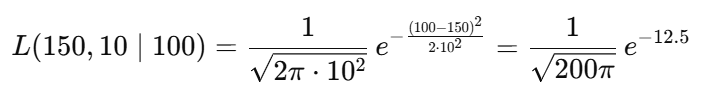
To compute the likelihood, we use the probability density function (PDF) of the normal distribution :

Plugging in the values :

This is a very small value, suggesting that :

Given a height of 100 cm, the likelihood that this data came from a normal distribution with μ = 150, σ = 10 is extremely low.

Varying the Data Point

Let’s see how likelihood changes as we change the observed height :

Height (x)	Likelihood L(μ = 150 , σ = 10 | x )	Interpretation
100 cm	1.47 × 10⁻⁷	Very unlikely under this distribution
130 cm	≈ 0.005	Still low, but more plausible
140 cm	≈ 0.2419	Much more likely
150 cm	≈ 0.3989(maximum)	Peak of the distribution
200 cm	≪ 0.005	Very unlikely

 As expected, likelihood is maximum when the observed data is equal to the mean of the distribution (i.e., 150 cm), and drops off as we move further away.

Final Insight: Probability vs Likelihood

Concept	What is Given	What is Being Evaluated	Type
Probability	Known distribution + parameters	Find the chance of observing an event	Forward
Likelihood	Known observed data (event)	Evaluate how well a parameter explains the observed data	Reverse

• Probability : You know the distribution and its parameters. You're finding how likely it is to observe a certain event.

• Likelihood : You observe the event (data), and you ask : How well does a certain parameter explain this data ?

Probability : This is a measure of the chance that a certain event will occur out of all possible events. It's usually presented as a ratio or fraction, and it ranges from 0 (meaning the event will not happen) to 1 (meaning the event is certain to happen).   

Likelihood : In a statistical context, likelihood is a function that measures the plausibility of a particular parameter value given some observed data. It quantifies how well a specific outcome supports specific parameter values.

More Definitions

A probability quantifies how often you observe a certain outcome of a test, given a certain understanding of the underlying data.  

A likelihood quantifies how good one's model is, given a set of data that's been observed.

Probabilities describe test outcomes, while likelihoods describe models.

Understanding Likelihood and Probability through Examples

We discussed three examples to understand the concept of likelihood and probability :

1. Coin Toss

2. Balls in a Bag

3. Normal Distribution

In all these cases, we deal with a parameter.

• In the coin toss example, the parameter is the probability of getting a head (say, p).

• In the balls in a bag example, the parameter might be the probability of drawing a green ball.

• In the normal distribution, the parameters are typically the mean (μ) and standard deviation (σ).

Let’s focus on the coin toss to understand likelihood in more depth.

Example : Coin Toss and Likelihood

Assume the probability of getting a head with a fair coin is p = 0.5 . Now, suppose we toss the coin 5 times and observe the outcome : HHHHH (i.e., 5 heads in a row).

We want to calculate the likelihood of observing this outcome under the assumption that the true probability of head is 0.5 .

This gives the likelihood of observing the data given the parameter p = 0.5 .

What if the Coin is Biased ?

Let’s assume the coin is slightly biased, and the probability of getting a head is p = 0.6.

Then the likelihood becomes :

Now compare :

This suggests that the data (5 heads in a row) is more likely under the assumption that p = 0.6 than p = 0.5.

Hence, the value p = 0.6 better explains the observed data.

Towards Maximum Likelihood Estimation (MLE)

Now, consider what value of p would maximize the likelihood of the observed outcome (HHHHH).

Clearly, if the coin is completely biased towards heads, i.e., p = 1, then :

This is the maximum possible value for likelihood in this scenario, since all heads are guaranteed when p = 1.

This leads us to the key idea :

Maximum Likelihood Estimation (MLE) is the process of choosing the parameter value that maximizes the likelihood of the observed data.

In our example, given the data HHHHH, the likelihood is maximized when p = 1 .

Key Concepts Recap

Probability : Given a model (i.e., a known p), what is the chance of observing a specific outcome ?

Likelihood : Given the observed data, how likely is a particular value of the parameter ? 

MLE : Find the parameter value that maximizes the likelihood of the observed data.

Maximum Likelihood Estimation (MLE) – Example 2

We have a bag that contains:

• 2 green balls

• 3 red balls

  So, the total number of balls = 5

The probability of drawing a green ball in a single draw (with replacement) is :

P(green) = 2/5

This scenario follows a Bernoulli distribution for each draw (success = green ball). Now, we perform 5 independent draws with replacement, and each time, we get a green ball. So, the observed data is :

G G G G G

Likelihood Calculation

Let’s define the parameter p as the probability of drawing a green ball.

We want to evaluate how well different values of p explain our observed data (GGGGG).

Case 1 : p = 2/5

Given this value of p, the likelihood of observing five greens in a row is :

Case 2 : p = 3/5

Clearly :

So, the likelihood is higher for p = 3/5 than for p = 2/5 , given the data.

Case  3 : p = 1

If we assume the probability of getting a green ball is 1 (i.e., all balls are green) :

Now ,

The value of p that maximizes the likelihood of observing the data is :

This is called the Maximum Likelihood Estimate (MLE) of p based on the observed data.

It means that given all 5 observed balls were green, the best explanation (highest likelihood) is that the bag only contains green balls — i.e., probability of green = 1 .

Conceptual Notes :

• Likelihood vs Probability :

  • Probability : Given a parameter value, what's the chance of some data ?

  • Likelihood : Given some data, how likely is a parameter value ?

• MLE always finds the parameter value that maximizes the likelihood of the observed data.

Example 3 : Maximum Likelihood Estimation in a Normal Distribution

Let’s consider a third example to understand Maximum Likelihood Estimation (MLE) more clearly.

Suppose we have a normal distribution with a mean μ = 150 and a standard deviation σ = 10.

Now, we randomly select one individual and observe that their height is 100. We want to evaluate how likely it is that this height of 100 came from the given normal distribution. This is where we calculate the likelihood of the observed data point under the specified distribution.

The likelihood function for a normal distribution is given by :

Substituting the values :

This value turns out to be very small, indicating that the observed data point (height = 100) is quite unlikely under the distribution with μ = 150 , σ = 10.

However, this does not mean that the data doesn't come from a normal distribution at all — it might be coming from a different normal distribution with a different mean and/or standard deviation.

So we ask : Which normal distribution makes this data point most likely ?

In other words, we try to find the parameters (like μ) of a normal distribution that maximize the likelihood of the observed data. This process is known as Maximum Likelihood Estimation (MLE).

In our example, clearly, a normal distribution with μ = 100 and the same σ = 10 would give the highest likelihood for the data point 100. So, under MLE, we would estimate that the mean μ of the distribution is 100 based on this observed data.

What is Maximum Likelihood Estimation ?

Maximum Likelihood Estimation (MLE) is a method for estimating the parameters of a statistical model. Given observed data, it finds the values of parameters that maximize the likelihood of the data under that model.

• In the coin toss example, we used the observed outcomes (e.g., HHHH or HTHT) to estimate the probability of heads p , such that the probability (likelihood) of the observed sequence is maximized.

• In the balls in a bag example, we found the proportion (or count) of colored balls that makes the observed draws most likely.

• In the normal distribution example, we estimated the mean μ that makes the observed height (100) most likely under a normal distribution.

In all cases, the observed data is fixed. The likelihood is treated as a function of the parameters, and we adjust those parameters to maximize the likelihood.

This is the core idea of MLE :

Find the parameter values that make the observed data most probable.

Understanding Maximum Likelihood Estimation with Normal Distribution

Recently, we discussed the concept of a normal distribution. Suppose we take a single random data point with a value of 100, and we know that it follows a normal distribution. If it indeed follows a normal distribution, then the most likely value of the mean (μ) is 100. At this point, the distribution achieves its maximum likelihood because the mean matches the data point exactly. In essence, maximum likelihood occurs when the value of μ equals the value of the observed data point.

However, a valid question arises: in real-world scenarios, we rarely deal with just one data point. Instead, we often have multiple observations. For example, assume we collect age data for 100 individuals. We determine that this dataset follows a normal distribution using techniques like the Shapiro-Wilk test, Q-Q plot, etc. But while we confirm the data follows a normal distribution, we don’t know which specific normal distribution it follows.

In other words, we don't know the actual values of the mean (μ) and standard deviation (σ). For instance, it could be a distribution where μ = 20 and σ = 5, or μ = 40 and σ = 5, or μ = 50 and σ = 3. These are all valid normal distributions but differ based on the values of μ and σ.

So, even if we know the data follows a normal distribution, the exact parameters (μ and σ) are unknown. A normal distribution is fully defined by its mean and standard deviation. To determine these parameters, we apply Maximum Likelihood Estimation (MLE).

Based on the observed data, we use MLE to estimate the values of μ and σ that maximize the likelihood function. In other words, we are trying to find the specific values of μ and σ that make the observed data most probable under the normal distribution. These estimates give us the best-fitting normal distribution for our dataset.

Strategy to Calculate Maximum Likelihood Estimation (MLE)

Let’s learn how to calculate the parameters (mean and standard deviation) using Maximum Likelihood Estimation (MLE).

We need to compute the likelihood :

We start by choosing random values for μ (mean) and σ (standard deviation).

For example :

• μ = 100

• σ = 10

Then we compute the likelihood for this pair :

Next, we change the value of σ and calculate the likelihood again :

We repeat this process for more combinations of μ and σ. Among all the computed likelihood values, we select the pair (μ, σ) that gives the maximum likelihood.

The values of μ and σ that maximize the likelihood function are our estimated parameter values.

This is the strategy we use to perform Maximum Likelihood Estimation.

Step 1 : Likelihood with a Single Data Point

Assume that for the time being, we do not have the entire dataset—only one data point , x₁​ .

The likelihood function is :

Step 2 : Likelihood with Multiple Data Points

Now, suppose we have multiple data points : x₁, x₂, x₃, ..., xₙ .

Only the x values change in the formula.

Let’s assume that all data points are independent.

Hence, the joint likelihood is the product of the individual likelihoods :

This expands to :

So if we have n independent observations, we multiply their individual likelihoods to get the overall likelihood.

Step 3 : Taking the Logarithm (Log-Likelihood)

To simplify this product, we take the natural logarithm of both sides :

Using the logarithmic identity log(ab) = log a + log b , the expression becomes :

We will now simplify one term, and since all terms follow the same pattern , the same simplification applies to all of them .

To find the best values of μ and σ , we compute the log-likelihood for different combinations of μ and σ. By evaluating the log-likelihood over a range (theoretically infinite) of values, we aim to identify the combination of μ and σ that maximizes the log-likelihood function.

If we have only one data point, say 100, we can try different normal distributions to evaluate how likely it is to observe that data point under each distribution:

• First, we try a normal distribution with some μ and σ, and the likelihood is low.

• Then, we try a second distribution, and the likelihood increases.

• After that, we try a third distribution, and the likelihood decreases again.

This pattern gives us an important insight. Imagine a graph where:

• The x-axis represents the value of μ .

• The y-axis represents the likelihood of the data under the normal distribution.

As we try different values of μ:

• When μ is small, the likelihood is low.

• As μ moves closer to the data point, the likelihood increases.

• After a certain point, increasing μ further causes the likelihood to decrease.

This implies that the graph of likelihood vs. μ has a maximum point—there is a peak in the curve.

To find this maximum point mathematically, we differentiate the log-likelihood function with respect to μ. The derivative represents the slope of the log-likelihood curve. The slope is zero at the maximum. So, to find the value of μ that gives us the highest likelihood, we solve :

This derivation shows that if we have n data points and we assume they follow a normal distribution, then the value of μ that maximizes the likelihood is simply the mean of the observed data points. This is a key result in Maximum Likelihood Estimation (MLE).

Now, we will apply the same logic to σ that we previously applied to μ .

We try different values of σ and observe how the shape of the normal distribution changes. Specifically, as σ changes, the width (spread) of the curve increases or decreases. Just like with μ, if we plot the likelihood as a function of σ, we will again observe a maximum point.

To find the value of σ that maximizes the likelihood, we again differentiate the log-likelihood function with respect to σ, set the derivative (slope) to zero, and solve for σ.

This means that the value of σ (standard deviation) which maximizes the likelihood is the standard deviation of the observed data.

So, if we are given a dataset (for example, a list of ages) and we assume it follows a normal distribution, then :

• μ is the mean of all data points.

• σ is the standard deviation of all data points.

These values are the maximum likelihood estimates of the parameters of the normal distribution.