Perceptron Loss Function: Overcoming the Perceptron Trick's Flaws
- Aryan

- Oct 27, 2025
- 7 min read
PROBLEM WITH PERCEPTRON TRICK
The biggest problem in the perceptron trick is that the values of coefficients are not necessarily the best values to classify between regions.
We cannot be certain that our chosen coefficients are the optimal ones that classify every point correctly.
If any point is misclassified, the perceptron algorithm adjusts the line so that this point is classified correctly.
However, if a point is already classified correctly, there is no change in the coefficients — meaning the line remains the same.
So:
For correctly classified points → no update to coefficients.
For misclassified points → coefficients are updated so that the line correctly classifies those points.
Main Flaws of the Perceptron Trick
Multiple possible separating lines:
We can often get many different lines that perfectly classify all the points. But how do we decide which line is better?
The perceptron trick doesn’t provide any metric or measure to tell which line gives the best classification.
No quantitative measure of performance:
The perceptron algorithm cannot tell how good a particular classification is.
It only focuses on correctly classifying points — not on how confidently or effectively it does so.
Hence, we can’t quantify the result.
Convergence issues:
The algorithm might fail to converge, especially when the data is not linearly separable.
It may keep adjusting the coefficients endlessly without reaching a stable solution.
In short, while the perceptron trick can classify points, it cannot guarantee convergence or identify the best possible line.
That’s why, in machine learning, we introduce the concept of a loss function — it allows us to quantify how good or bad our current solution is and helps us find the optimal line systematically.
PERCEPTRON LOSS FUNCTION
A loss function is simply a mathematical tool that helps us measure how far our model’s predictions are from being correct.
It depends on the coefficients of the line (or model). For every possible set of coefficients, the loss function gives us a number that represents how much error our model currently has.
Whenever we draw a line, we can calculate its loss — and as we keep changing the line’s coefficients, this value also changes.
In the perceptron, the general loss function can be written as:

Here:
n is the number of data points.
L(yᵢ, f(xᵢ)) measures the individual loss for each data point.
R(w₁, w₂) is the regularization term (used to prevent overfitting), and α controls its strength.
For now, we’re not using regularization, so we’ll drop that term and focus only on the core part of the perceptron loss.
Simplified Form
In the perceptron, the loss for each point is defined as:
L(yᵢ,f(xᵢ)) = max(0,−yᵢf(xᵢ))
Where
f(xᵢ) = w₁xᵢ₁ + w₂xᵢ₂ + b
This means the loss is zero if the point is correctly classified (because yᵢ f(xᵢ) > 0),
and positive if the point is misclassified (because yᵢ f(xᵢ) < 0).
Putting everything together:

Here 1\n simply means we are taking the average loss across all points.
This value changes only when we adjust the coefficients w₁ , w₂ , b — since xᵢ and yᵢ are constants from our dataset.
Our aim is to find those values of w₁ , w₂ , b that make the total loss as small as possible:

We try different combinations of weights and bias until we reach the one that gives the minimum possible loss, meaning our model is classifying the data as correctly as it can.
Explanation of Loss Function
Now let’s understand what the loss function means and what it is trying to express.

Where
f(xᵢ) = w₁xᵢ₁ + w₂xᵢ₂ + b
and our dataset is represented as:
x₁ | x₂ | y |
x₁₁ | x₁₂ | y₁ |
x₂₁ | x₂₂ | y₂ |
... | ... | ... |
Here, there are n data points, and we represent each input feature as xᵢⱼ .
Breaking Down the Loss Function
The key term inside the loss function is:
max(0, −yᵢ f(xᵢ))
Let’s take −yᵢ f(xᵢ) = x
Then, according to the max function rule:
If x ≥ 0, then max(0,x) = x
If x < 0 , then max(0,x) = 0
So,
max(0, −yᵢ f(xᵢ))
means:
If −yᵢ f(xᵢ) ≥ 0, the output is −yᵢ f(xᵢ)
If −yᵢ f(xᵢ) < 0 , the output is 0
That’s the basic intuition behind this part of the function.
Example for Two Points
Let’s simplify the formula assuming we only have two data points:

Here,
f(x₁) = w₁x₁₁ + w₂x₁₂ + b
f(x₂) = w₁x₂₁ + w₂x₂₂ + b
If we had n points, we would simply keep adding more terms inside the summation.
Geometric Intuition
Let’s build an intuition for how the loss function works geometrically.
We have a small dataset of students with their CGPA and IQ values, and the target variable indicates whether they are placed (1) or not placed (-1).
CGPA | IQ | Placed |
7 | 8 | 1 |
6 | 8 | -1 |
4 | 2 | 1 |
1 | 1 | -1 |
Here:
Green points → Students who got placed (y = 1)
Red points → Students who were not placed (y = -1)
When we draw a decision line, each point can fall into one of four categories:
Actual (yᵢ) | Predicted (ŷ) | Case Description |
1 | 1 | Correct: placed → placed |
-1 | -1 | Correct: not placed → not placed |
1 | -1 | Misclassified: placed → not placed |
-1 | 1 | Misclassified: not placed → placed |
Now, let’s see how the loss function term
max(0, -yᵢf(xᵢ))
behaves for each point.
yᵢ | ŷ | max(0, -yᵢf(xᵢ)) |
1 | 1 | 0 |
-1 | -1 | 0 |
1 | -1 | non-zero |
-1 | 1 | non-zero |
Why This Happens
Let’s analyze it intuitively:
For a correctly classified positive point (green),
f(xᵢ) = w₁x₁ + w₂x₂ + b > 0,
and yᵢ = 1 .
So, −yᵢ f(xᵢ) becomes negative, and
max(0,negative value) = 0
Hence, no loss is added.
For a correctly classified negative point (red),
f(xᵢ) < 0 and yᵢ = −1
So, −yᵢ f(xᵢ) again becomes negative,
giving a 0 loss.
For misclassified points, yᵢ f(xᵢ) becomes negative,
making −yᵢ f(xᵢ) positive, so the loss term becomes non-zero.
Conclusion
Correctly classified points → contribute 0 to the total loss.
Misclassified points → contribute a positive value to the loss.
This means the loss function directly measures how many points are misclassified and how strongly they are misclassified.
Geometrically, the value of f(xᵢ) = w₁x₁ + w₂x₂ + b gives a proportional measure (not exact distance) of how far a point lies from the separating line.
Hence, our goal is to find the values of coefficients (w₁, w₂, b) that make the total loss minimum.
Gradient Descent
We want to minimize our loss function with respect to the coefficients w₁, w₂, and b:
Where
f(xᵢ) = w₁xᵢ₁ + w₂xᵢ₂ + b
We need to find the values of w₁, w₂, and b that make the loss function minimum.
To achieve this, we use an optimization technique called Gradient Descent.
The loss function depends on the three parameters — w₁, w₂, b .
If we change any of these values, the loss will also change.
Hence, our goal is to adjust these parameters in the direction that reduces the loss the most.
Gradient Descent Process
Initialize
Start with random values of w₁, w₂, and b, for example w₁ = 1, w₂ = 1, b = 1 .
Choose Learning Rate
Select a small constant η , known as the learning rate.
Typical values are around 0.01.
Iterate for Multiple Epochs
Repeat the update process for a fixed number of epochs (iterations).
Update Rules
After computing gradients (partial derivatives), update parameters as follows:

Partial Derivatives
The loss function involves the term max(0, −yᵢ f(xᵢ)) , which is not differentiable everywhere,
but we can handle it using the chain rule and conditional derivatives.

We know:
f(xᵢ) = w₁xᵢ₁ + w₂xᵢ₂ + b
And

Combining these, we get :
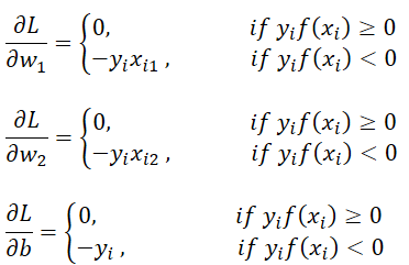
During each epoch, we calculate these gradients for all data points and update w₁, w₂, b accordingly.
Step by step, the model moves toward values that reduce the overall loss.
After enough iterations, we reach a set of parameters where the loss is minimum,
meaning our line (decision boundary) now classifies the data as accurately as possible.
More Loss Functions
We know that a perceptron is essentially a mathematical model.
It takes inputs, multiplies them by corresponding coefficients (weights), adds them up, and finally passes the result through an activation function to produce an output.
This design is very flexible, which is why the perceptron can be adapted for different types of problems just by changing the activation function and loss function.
1. Binary Classification (Step Activation – Perceptron)
In the classic perceptron, we use a step activation function, which outputs either 1 or -1.
The corresponding loss function used here is the hinge loss or perceptron loss.
This setup is used for binary classification.
2. Binary Classification (Sigmoid Activation – Logistic Regression)
Sometimes, instead of a hard 1 or -1 output, we may want probabilities (values between 0 and 1).
In that case, we replace the step activation with the sigmoid function.
When we use the sigmoid activation, our output becomes a probability, and we use binary cross-entropy (log loss) as the loss function.
This combination — sigmoid activation + binary cross-entropy loss — is exactly what we use in logistic regression.
Technically, the perceptron becomes equivalent to logistic regression when we use a sigmoid activation and binary cross-entropy loss.
3. Multi-Class Classification (Softmax Activation)
If we want to classify more than two classes, we can extend this concept.
Instead of sigmoid, we use the softmax activation function, which gives probabilities across multiple classes that sum to 1.
In this case, the suitable loss function is categorical cross-entropy.
So:
Activation: Softmax
Loss Function: Categorical Cross-Entropy
Use Case: Multi-class classification
4. Regression (Linear Activation)
We can also use the perceptron for regression problems.
For that, we simply use a linear activation function (no nonlinearity) and the Mean Squared Error (MSE) loss function.
So:
Activation: Linear
Loss Function: MSE
Use Case: Regression (e.g., Linear Regression)
In short, the perceptron is a general mathematical framework.
By simply swapping out the activation and loss functions, it can behave as a classifier or regressor, depending on what the task demands.
That’s what makes it so flexible — and the foundation for all neural networks that followed.


