The Core Math Behind XGBoost
- Aryan
- Aug 26, 2025
- 9 min read
XGBoost Objective Function
Suppose we have data of students:
cgpa | iq | package |
6.5 | 71 | 13 |
5.0 | 91 | 10 |
9.1 | 120 | 16 |

Output Formula :

Let's see the process behind how this formula is derived.
Step 1: Model Combination
The combined XGBoost model has two models m₁ and m₂ .
The total prediction is the sum of outputs from the first and second models:

In functional form:

Here, f₁(xᵢ) is the prediction from the first model. In our case, it always outputs 13 (the mean).
Now, we need to compute the output of the second model. Since we have three leaf nodes, we must calculate three output values.
In general, for t models:

Step 2: Defining the Loss Function
The goal of any model is to make predictions ŷᵢ as close as possible to the actual values yᵢ .
To measure this difference, we use a loss function.
For regression, a common choice is Mean Squared Error (MSE):

Our task is to minimize this loss function.
Gradient Boosting is flexible—it can work with any differentiable loss function. However, XGBoost modifies this loss by adding built-in regularization, which controls model complexity.
Step 3: XGBoost Objective Function
With two models (m₁,m₂) , the objective function becomes :

where the regularization term is :

T: number of leaf nodes in the decision tree
wⱼ : weight (output) of leaf node j
γ , λ : regularization parameters
Unlike plain Gradient Boosting, XGBoost has built-in regularization.
This means instead of only minimizing the loss function, it also penalizes overly complex trees.
Our task is to find the optimal leaf weights (wⱼ) that minimize the objective function.
The Derivation
The objective function in XGBoost can be written as:

This is called the objective function because it has two parts:
Loss function L(yᵢ ,ŷᵢ), which measures prediction error.
Regularization term Ω(fₜ (xᵢ)) , which controls model complexity.
We’ll study how this function evolves as we add models in a stagewise manner. Starting with a simple mean model, we then keep adding decision trees and observe how the objective function changes.
Stage 1: Single Model (Mean)
At first, we only have one model m₁ , which is simply the mean of the output column.
Since this is not a decision tree, the regularization term does not apply.
Thus, the objective reduces to:

Stage 2: Mean + One Decision Tree
Now we introduce a second model — a decision tree.
The prediction becomes:
ŷᵢ = f₁(xᵢ) + f₂(xᵢ)
Since a decision tree is added, we now apply the regularization term to it :

Stage 3: Mean + Two Decision Trees
Next, we add another decision tree. Our prediction is:
ŷᵢ = f₁(xᵢ) + f₂(xᵢ) + f₃(xᵢ)
So the objective becomes:

Stage t: General Case
At stage t , we have the mean model plus (t−1) decision trees.
The prediction is:
ŷᵢ = f₁(xᵢ) + f₂(xᵢ) + ....+ fₜ(xᵢ)
Thus, the objective becomes:

Compact Form
This can also be written more compactly as:

where ŷᵢ⁽ᵗ⁻¹⁾ represents the prediction from all previous models (stages 1 to t−1).
Our goal is to find the function fₜ(xᵢ) that minimizes this objective.
In other words, XGBoost transforms the problem into an optimization task: adding one model at a time to reduce the overall loss while controlling complexity.
Taylor’s Series Expansion
We have transformed the optimization problem into the following form :

The Challenge: Non-Differentiable Loss Surface
Optimizing this function is tricky because the surface is not smooth, unlike linear regression. Since decision trees are involved, the resulting curve is zigzagged and irregular. When plotted, the loss function produces a surface that is difficult to optimize due to:
Non-differentiable points – At many points, the function cannot be differentiated.
No clear slope – Partial derivatives cannot be applied since we cannot define a tangent slope.
Discontinuities – The tree structure introduces step-like jumps in the function.
Previously, we used partial derivatives to find optimal values, but in this case the loss curve is often non-differentiable. This prevents us from finding slopes and thus makes minimizing the objective function through traditional calculus-based methods impossible.
Smoothing with Taylor Series
What if we could smooth or approximate this irregular curve? Imagine replacing the complex function with one that is:
Very close in value
Smooth and continuous
Differentiable with respect to fₜ(xᵢ)
To do this, we approximate the term :

using a Taylor series expansion.
This transforms the optimization problem from dealing with an irregular, discontinuous surface into one with a smooth, differentiable polynomial approximation. Such a curve can then be optimized using standard calculus techniques.
THE SOLUTION - TAYLOR SERIES
Taylor series is a very powerful approximation technique. It says: take any complex mathematical function, and Taylor series can approximate it using a polynomial. It can approximate complex mathematical functions using simple polynomials. This is the core definition. If you input a complex function, you will be able to approximate it using polynomials. This is the main idea behind Taylor series.
Key principle: If you want accurate approximation, the polynomial will have many terms. The more polynomial terms we add, the better it will approximate the complex function.
Taylor Series Formula
Taylor series uses derivatives to convert any complex function into a polynomial. Around point a:

The more derivative terms we add, the more accurate our approximation becomes.
Example: Approximating eˣ around a = 0
Let's work through the Taylor series expansion of f(x) = eˣ at a = 0 :
Step 1: Calculate function and derivatives at a = 0

Step 2: Build the Taylor series

Final approximation:

Visual Understanding
The graphs show how adding more terms improves the approximation:
1st order: f(x) ≈ 1 + x (linear approximation)

2nd order: f(x) ≈ 1 + x + x²/2 (quadratic approximation)

3rd order: f(x) ≈ 1 + x + x²/2 + x³/6 (cubic approximation)

As we can see from the graphs, each additional term makes our polynomial approximation closer to the original function over a wider range of values.
The Magic of Taylor Series
The more terms we add to this polynomial, the better our approximation accuracy becomes. This is the magic of Taylor series - it transforms complex, non-differentiable functions into smooth, differentiable polynomials that we can easily work with mathematically.
APPLYING TAYLOR SERIES
Now we will apply Taylor series to our objective function:

We will apply Taylor series expansion up to the second degree polynomial. We will apply it specifically to the loss function part: ∑ᵢ₌₁ⁿ (yᵢ, ŷᵢ⁽ᵗ⁻¹⁾ + fₜ(xᵢ))
Setting up the Taylor Series
Recall the general Taylor series formula:

For our application:
x = ŷᵢ⁽ᵗ⁻¹⁾ + fₜ(xᵢ) (current prediction)
a = ŷᵢ⁽ᵗ⁻¹⁾ (prediction from previous models)
(x−a) = fₜ(xᵢ) (contribution of new model)
Calculating Each Term
Term 1: f(a)

Term 2: First derivative term

Term 3: Second derivative term

Introducing Gradient and Hessian
To simplify notation, we define:

Final Simplified Objective Function
Substituting our gradient and hessian notation:

This is our simplified objective function after applying Taylor series approximation.
The key achievement here is that we've transformed our complex, non-differentiable objective function into a smooth quadratic function in terms of fₜ(xᵢ) , which we can now optimize using standard calculus techniques.
SIMPLIFICATION
Starting with our Taylor series approximated objective function:

We need to find the value of fₜ(xᵢ) that minimizes this objective function. Our plan is to differentiate this with respect to fₜ(xᵢ) and set it equal to zero.
When we differentiate with respect to fₜ(xᵢ) , the term L(yᵢ , ŷᵢ⁽ᵗ⁻¹⁾) becomes zero since it's a constant (independent of fₜ(xᵢ)) .
Therefore, we can simplify our objective function to:

Expanding the Regularization Term
Now we expand the regularization term Ω(fₜ(xᵢ)) . Assuming our current decision tree has T leaf nodes, the regularization term becomes:

Which can be written more compactly as :

Substituting this back into our objective function:

Rearranging Summations
Currently, we have two different summation indices:
Index i from 1 to n (number of data points/rows)
Index j from 1 to T (number of leaf nodes)
To optimize this function, we need to align these summations. We'll rearrange by grouping terms according to leaf nodes rather than data points.
Key transformation -
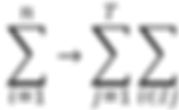
Where Iⱼ represents the set of data points that fall into leaf node j .
This gives us:

Where:
wⱼ = fₜ(xᵢ) for all data points xᵢ that fall into leaf node j
Iⱼ is the instance set (collection of data points) assigned to leaf node j
This transformation allows us to optimize the objective function with respect to each leaf node weight wⱼ independently.
Understanding the Summation Transformation
Let's understand how this transformation happens by examining the summation transformation process. Consider a dataset of students with CGPA and placement package information:
cgpa (xᵢ) | package (yᵢ) |
7.1 | 4.5 |
8.2 | 6.9 |
6.5 | 5.1 |
9.1 | 10 |
We start with our objective function:

And we need to transform it to:

Step-by-Step Transformation
If we expand the first equation for our four data points, we get:

This gives us four terms, one for each data point. Now, when we build our decision tree, suppose:
Leaf node 1: Contains row 3 (CGPA = 6.5)
Leaf node 2: Contains rows 1, 2, and 4 (CGPA = 7.1, 8.2, 9.1)
The outer summation expands over the two leaf nodes, where i∈Iⱼ represents the instance set of leaf j. Reorganizing by leaf nodes:

Equations (1) and (2) are identical—only the order differs. We're performing the same computation but organizing it according to the decision tree structure.
Understanding the Notation Change: fₜ(xᵢ) to wⱼ
The key insight is that fₜ(xᵢ) represents the output of the decision tree for data point i, but all points in the same leaf node receive the same output value. Therefore:
For row 3 in leaf node 1: fₜ(x₃) = w₁
For rows 1, 2, 4 in leaf node 2: fₜ(x₁) = fₜ(x₂) = fₜ(x₄) = w₂
Where wⱼ is the output value for leaf node j. Substituting this into equation (2):

Final Simplified Objective Function
Now we can rewrite our objective function in its simplified form:

Combining the regularization terms:

Factoring out common terms:

Optimization: Finding the Optimal Weights
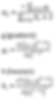
Now we can differentiate this objective function with respect to wⱼ to find the optimal leaf weights:

Solving for wⱼ :

This formula gives us the optimal output value for each leaf node j , where we need to calculate the gradients gᵢ and Hessians hᵢ based on our specific loss function.
Output Value for Regression
We know

So we need gᵢ (gradient) and hᵢ (hessian).
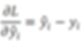
Definitions

These depend on the chosen loss. For regression, we typically use mean squared error (MSE):

Differentiate w.r.t. ŷᵢ :
At iteration t , this is evaluated at the previous prediction ŷᵢ⁽ᵗ⁻¹⁾ . Hence

Therefore

which is the sum of residuals in leaf j .
Now the Hessian: differentiating again,

So the denominator becomes

i.e., number of points in the leaf plus the regularization term.
Putting it together,

So the leaf output for regression is

where N is the count of samples falling into that leaf.
(Example intuition: the first model is usually the mean; after predicting with it we add a new tree. Its leaf weights wⱼ are just the average residuals in each leaf, shrunk by λ .)
Output Value for Classification
In the classification scenario, to calculate gradient and hessian we differentiate and double-differentiate the loss function.
Here, the loss function is log loss.
The expression for wⱼ is similar to the regression case, but the denominator changes for classification.
The first derivative (gradient) is:
gᵢ = (yᵢ − pᵢ)
which we can also call the residual, where pᵢ is the predicted probability from the previous iteration.
The second derivative (hessian) is:
hᵢ = pᵢ(1 − pᵢ)
again taken from the probability of the previous iteration.
Thus,

where pᵢ is the predicted probability at the previous iteration or timestamp.
DERIVATION OF SIMILARITY SCORE
We start from the per-iteration objective

and the optimal leaf weight

Substitute wⱼ back into the objective to get the minimum value contributed by the t-th tree:

This is the minimum objective value after adding the t-th tree.
It also gives a natural node quality measure (often called the similarity score for a leaf j):

More negative contributions reduce the objective more, meaning a better leaf/structure.
This score can replace impurity measures like Gini/entropy when evaluating tree structure quality in XGBoost.
Final Calculation of Similarity
The similarity score for the whole tree is:

Now, we can substitute the actual values of gᵢ and hᵢ :
Regression:
gᵢ is the residual (derivative of loss w.r.t prediction).
hᵢ = 1.
When we sum over samples in a leaf, ∑hᵢ = number of samples in that leaf.
Classification (logistic):
gᵢ = yᵢ - pᵢ , i.e., again the residual.
hᵢ = pᵢ(1 - pᵢ) , the variance of the Bernoulli distribution.
So, plugging these into the similarity formula directly gives us the respective formulas for regression and classification trees.
Tree Building Using Similarity Score
We start with the objective function at iteration t :

Step 1: Single Leaf (Parent Node)
At the beginning, we have a single leaf node p :

This is the similarity score for the parent node.
Step 2: Splitting into Two Leaves
When we split the node into left (L) and right (R) children, the new objective becomes :

Step 3: Loss Reduction from the Split
The gain (reduction in loss) from splitting is:

Substituting:

After simplification:

This final formula tells us whether a split is useful:
If Gain > 0, the split reduces loss and is accepted.
If Gain ≤ 0, the split is not beneficial.
Intuition
The numerator (∑gᵢ)² measures how strong the gradients are in a region → larger values mean the split is capturing a stronger signal.
The denominator (∑hᵢ + λ) acts like a regularizer → it prevents the model from making splits that are too sensitive to noise.
The term γ is the cost of creating an additional leaf → it forces the model to only create a new split if the reduction in loss is worth the added complexity.
So in simple words: XGBoost prefers splits that create leaves with concentrated gradients (strong signals), while avoiding splits that just add complexity without much gain.