DECISION TREES - 1

INTRODUCTION

Decision trees stand out as a versatile and intuitive approach in machine learning. Being non-parametric, they make no assumptions about the underlying data distribution, allowing them to effectively model non-linear data relationships. As a white box model, their decision-making process is transparent and easily interpretable, offering valuable insights into the factors influencing predictions. Often considered the mother of all tree-based algorithms, the fundamental principles of decision trees lay the groundwork for more advanced ensemble methods. Notably, they are adaptable and work with both classification and regression tasks, making them a powerful tool for a wide range of predictive modeling problems.

INTUTION BEHIND DECISION TREES

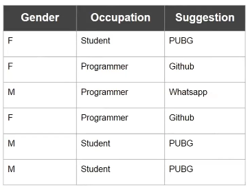
Imagine you're trying to recommend an app to a user based on their Gender and Occupation, just like in the dataset we have. For a moment, let's forget about machine learning and think logically. If a new customer tells us their gender and occupation, how would we decide which app to suggest based on the patterns in our existing data?

Looking at the data, a clear set of rules emerges :

• If the Occupation is "Student", then we should suggest "PUBG".

• If the Occupation is "Programmer", then we need to consider their Gender:

  • If the Gender is "Male", then we suggest "Whatsapp".

  • Else (if the Gender is "Female"), then we suggest "Github".

This sequence of "if" conditions, where the outcome of one condition leads to another, is precisely the fundamental idea behind a decision tree. It's essentially a giant nested if-else structure that learns these decision rules directly from the data.

This intuitive approach of making sequential decisions based on different attributes is what makes decision trees so understandable and powerful. The next step is to visualize how this logical flow translates into the tree structure we often see.

Visualizing the Decision Tree Structure

You've correctly identified that the nested if-else rules form the basis of a decision tree. The reason we call it a "tree" is because this sequential decision-making process can be naturally represented as a hierarchical structure, much like an upside-down tree.

Imagine starting at the top. The first decision we made was based on the Occupation. This becomes the root node of our tree.

• From the root node ("Occupation"), branches extend based on the possible values of this attribute: "Student" and "Programmer".

• If the Occupation is "Student", we directly arrive at the suggestion "PUBG". This becomes a leaf node, representing the final prediction for this branch.

• If the Occupation is "Programmer", we then made a decision based on Gender. So, from the "Programmer" branch, we have another internal node representing the "Gender" attribute.

• From the "Gender" node, two more branches extend based on its values: "Male" and "Female".

• The ends of these branches lead to the final suggestions: "Whatsapp" for "Male" and "Github" for "Female". These are also leaf nodes.

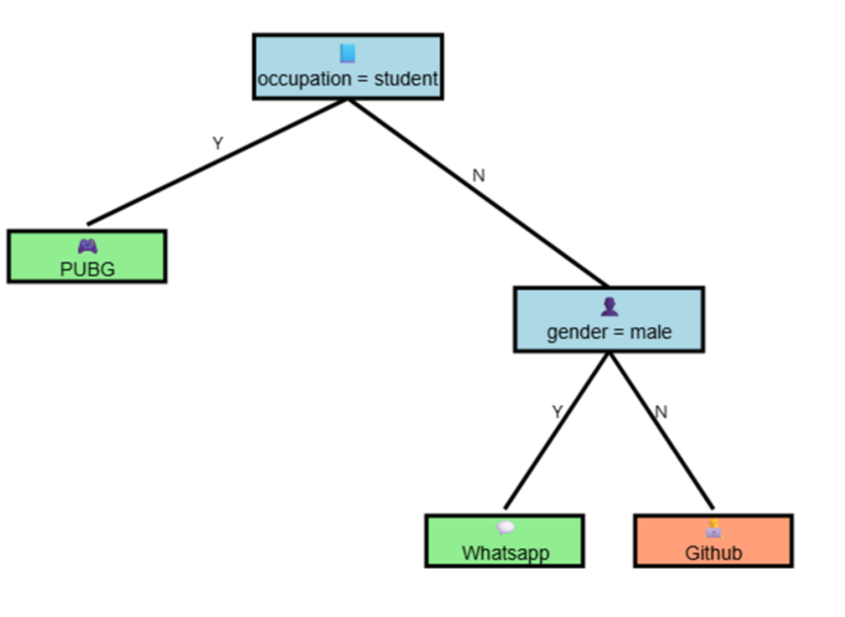
By visualizing the decision process in this way, the "tree" terminology becomes clear. Each node represents a decision point (a test on an attribute), each branch represents the outcome of that decision, and the leaves represent the final predictions. This hierarchical structure makes the decision-making process transparent and easy to follow.

Example 2

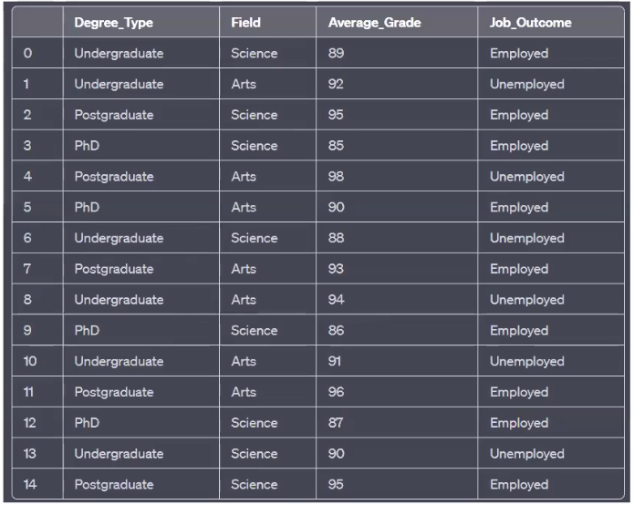
Consider the task of predicting Job_Outcome based on Degree_Type, Field, and Average_Grade, as presented in the subsequent dataset. While the underlying principle of creating a predictive model through a series of decisions remains the same as in the simpler app recommendation example, the process of manually defining the optimal sequence of decisions and the corresponding tree structure becomes considerably challenging, even with this moderately sized dataset.

In real-world scenarios, datasets often encompass hundreds or even thousands of input features. Manually discerning the most relevant features and their optimal splitting points to create an effective decision tree under such conditions is a practically insurmountable task.

Therefore, the power and utility of decision trees in machine learning are intrinsically linked to the algorithms that automate their construction. These algorithms, such as ID3, C4.5, and the CART (Classification and Regression Trees) algorithm that will be the focus of further discussion, employ computational methods to :

• Identify the most informative features: Algorithms assess each input feature to determine which one best separates the data with respect to the target variable.

• Determine optimal split thresholds: For both categorical and continuous features, algorithms find the values or ranges that create the most distinct groups in terms of the target variable.

• Manage tree complexity: Algorithms incorporate mechanisms to control the size and structure of the tree to prevent overfitting and ensure good generalization performance on unseen data.

CART, with its capacity for both classification and regression tasks and its implementation in the widely used scikit-learn (sklearn) library, exemplifies such an automated approach. These algorithms abstract away the manual complexity of building decision trees, enabling their effective application to a wide range of machine learning problems involving intricate datasets.

VOCAB

 THE CART ALGORITHM - CLASSIFICATION

CART stands for Classification and Regression Trees. It is an algorithm used to construct decision trees for both classification and regression tasks.

Let’s consider a dataset that contains n input features and one output column. Suppose the output column is categorical—that is, it contains values like "Yes" and "No". The input features, however, can be of any data type (numerical, categorical, etc.).

Our objective is to train a decision tree model that, based on the input data, can accurately predict the output.

Structure of a Decision Tree

A decision tree is composed of different types of nodes:

• Root Node: The starting point of the tree; represents the entire dataset and the first decision.

• Decision Nodes: Internal nodes where the data is split based on certain criteria.

• Leaf Nodes: Terminal nodes that represent the final output or prediction (e.g., "Yes" or "No").

To construct a tree, we repeatedly create nodes by splitting the dataset based on specific conditions. This process is called splitting, and it's driven by a splitting criterion.

Node Creation and Splitting Criteria

At each node, the algorithm must decide how to split the data. This is done using a splitting criterion, which consists of two components :

1. A selected feature fᵢ , where i ∈ {1,2,...,n}

2. A threshold value θ a, which is used to divide the data

So, the splitting criterion can be denoted as:

                                           θ → (fᵢ , value)

This means we choose a feature fᵢ , and a specific value of that feature, and use it to divide the dataset. For example :

• If fᵢ is a numerical feature, the split might be :

  If fᵢ ≤ θ go left, else go right

• If fᵢ is a categorical feature, the split might be :

  If fᵢ = "Category A" go left, else go right

This process is repeated recursively, creating more nodes, until a stopping condition is met (e.g., maximum depth, pure class in a node, minimum number of samples).

How a Decision Tree Chooses the Best Split

How Do We Choose the Best Split?

The key challenge is :

Out of all possible features and their values, how do we decide the best feature and value for splitting?

The approach is exhaustive search:

• Try every feature f₁ , f₂ , … , fₘ

• For each feature, try every unique value in that column as a potential split point

For each (feature, value) pair :

1. Split the data into D₁ and D₂

2. Calculate an impurity measure

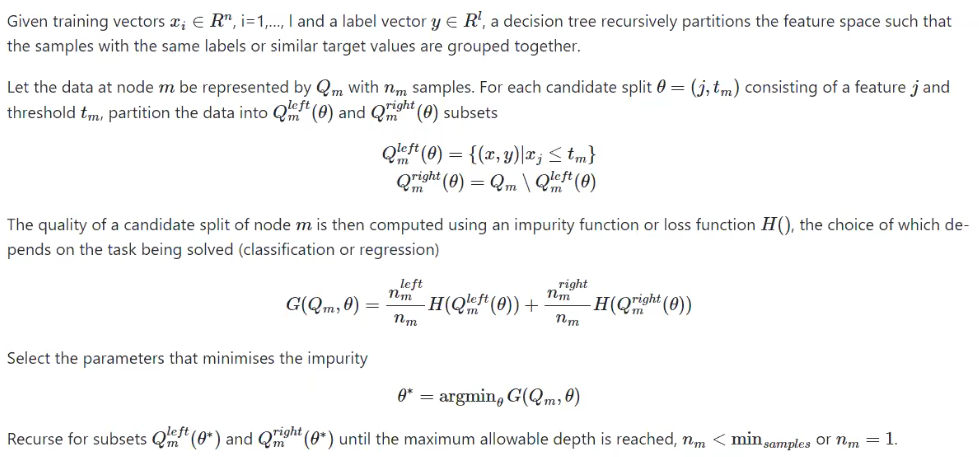
Impurity Function

To evaluate the "quality" of a split, we use an impurity function, denoted as H().

• For classification tasks, common impurity functions are:

  • Gini Impurity

  • Entropy

• For regression tasks, we typically use:

  • Mean Squared Error (MSE)

  • Mean Absolute Error (MAE)

After splitting the data, we compute the impurity for each child node :

Since the number of rows in D₁ and D₂ may differ, we calculate a weighted average of the impurity :

Here , G is the overall impurity score for a given (feature, value) split .

Selecting the Best Split

• Compute G for every possible (feature, value) pair

• Select the pair with the minimum G — this gives the best split

• Use this pair to create the current node

• Recursively repeat this process on the resulting subsets D₁ and D₂

When to Stop Splitting

Splitting continues recursively until a stopping condition is met. Common stopping criteria include:

• All rows in the node belong to the same class

• A maximum tree depth is reached

• The number of rows in the node is below a predefined threshold

• No further meaningful splits can be made (e.g., all features are constant)

Once a node can no longer be split, it becomes a leaf node, which holds the final prediction.

Splitting Categorical Features in Decision Trees

We are dealing with a classification problem where our goal is to predict the Job_outcome (Employed or Unemployed) based on other input features like Degree_type, Field, and Average_Grade.

What are we trying to do?

We are trying to build a Decision Tree to classify whether a student is likely to be Employed or Unemployed. The very first step is to choose the best feature to split on at the root.

How Do We Choose the Best Feature?

We use Gini Impurity to measure how "pure" or "impure" a node is.

Gini Impurity Intuition:

• Gini impurity measures the probability of misclassifying a randomly chosen element if we label it according to the distribution in a group.

• Lower Gini = Better split (purer groups)

• If all examples in a node belong to the same class → Gini = 0 (perfectly pure)

• If classes are evenly mixed → Gini is highest (closer to 0.5 for binary)

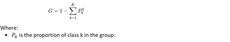
Gini Formula :

Step-by-Step : Splitting on field Column

Step 1 : Identify it as a Binary Feature

Field has two unique values: Science and Arts

We split the data into two groups:

• Group 1 → Field = Science

• Group 2 → Field ≠ Science (i.e., Arts)

Step 2: Count Job Outcomes in Each Group

Group 1: Field = Science

Row	Job Outcome
0	Employed
2	Employed
3	Employed
4	Unemployed
9	Employed

• Employed = 4

• Unemployed = 1

Group 2: Field = Arts

Row	Job Outcome
1	Unemployed
5	Employed
7	Unemployed
8	Unemployed
6	Employed

• Employed = 2

• Unemployed = 3

Step 3 : Calculate Gini for Each Group

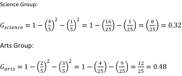
Step 4: Calculate Overall (Weighted) Gini Impurity

Since both groups have 5 records, we assign equal weight :

Final Gini for split on field = 0.40

What Next?

This value (0.40) is now compared with Gini values from splits on other features like:

• degree_type = Undergraduate, Postgraduate, or PhD

• average_grade with various thresholds (e.g., >= 90)

Whichever feature + value combination gives the lowest Gini will be used as the root node .

Why We Do This:

• Decision trees are greedy algorithms—they pick the best feature to split on at each step, aiming to maximize purity (minimize impurity) after the split.

• The root node has the biggest impact, so we want to pick the best possible feature here.

Summary

• We started with field because it’s a simple binary feature.

• We calculated Gini impurity for both resulting groups.

• We used weighted average to get the total impurity for that split.

• Final Gini = 0.4 for field.

• We'll repeat this process for other features to compare and choose the best root.

Splitting on Categorical Features in Decision Trees

In decision tree classifiers, choosing the best feature to split on is critical for building a pure and accurate model. Here's a deep dive into how to evaluate a categorical multiclass feature—Degree_Type—using Gini impurity to determine the most effective binary split.

Problem Context

We are working with a small educational dataset of 10 students. Each student has the following features :

• Degree_Type (Undergraduate, Postgraduate, PhD)

• Field (Science, Arts)

• Average_Grade (numerical)

• Job_Outcome (Employed or Unemployed — our target variable)

Our goal is to determine how to split the data on the Degree_Type feature to best separate the outcomes (Employed vs Unemployed) using Gini impurity.

Step-by-Step : One - vs - Rest Splits for Degree_Type

Since Degree_Type is a categorical feature with three unique values, we perform One-vs-Rest binary splits for each :

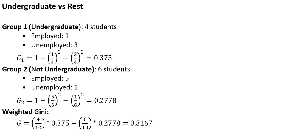
• Undergraduate vs Not

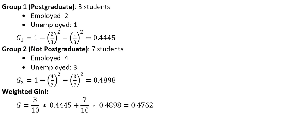
• Postgraduate vs Not

• PhD vs Not

Data Summary

Degree_Type	Job Outcome	Count
Undergraduate	Employed: 1	4
	Unemployed: 3
Postgraduate	Employed: 2	3
	Unemployed: 1
PhD	Employed: 3	3
	Unemployed: 0
Total		10

Split Evaluations

Postgraduate vs Rest

PhD vs Rest

Conclusion

Split Type	Weighted Gini
Undergraduate vs Rest	0.3167  Best
PhD vs Rest	0.3429
Postgraduate vs Rest	0.4762

Undergraduate vs Rest provides the purest binary split for the Degree_Type feature, making it the best candidate if this feature is chosen for the root or a node in the decision tree .

Splitting Numerical Features in Decision Trees

Why Not One-vs-Rest?

For categorical features, decision trees can use one-vs-rest or multiway splits.

But for numerical features, we cannot split by individual values or categories. Instead, we use threshold-based binary splits of the form:

                Average_Grade ≤ θ vs Average_Grade > θ

Step 1 : Sort the Data by Average_Grade

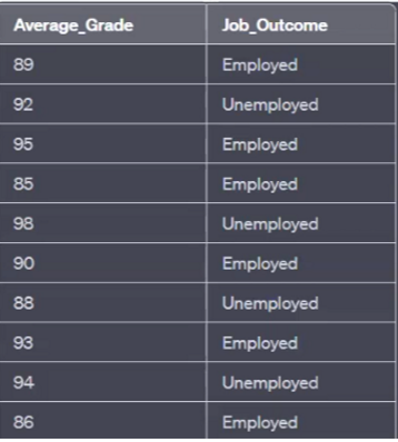
We start by sorting the data points in ascending order of Average_Grade :

Average_Grade	Job_Outcome
85	Employed
86	Employed
88	Unemployed
89	Employed
90	Employed
92	Unemployed
93	Employed
94	Unemployed
95	Employed
98	Unemployed

Step 2: Identify Candidate Thresholds (Split Points)

Calculate midpoints between each pair of consecutive grades:

Candidate split thresholds (θ) :

85.5, 87.0, 88.5, 89.5, 90.5, 92.0, 93.5, 94.5, 96.5

Each θ divides the dataset into two parts :

• Left Node: Average_Grade ≤ θ

• Right Node: Average_Grade > θ

Step 3: Evaluate Gini Impurity at Each Split

Example : Split at θ = 85.5

Split Rule :

• Left: Grades ≤ 85.5 → 1 sample → [Employed] → Pure → Gini = 0

• Right: Grades > 85.5 → 9 samples

  • Employed = 5

  • Unemployed = 4

Gini Impurity Formula for a node :

Step 4 : Repeat for All Candidate Splits

For each split θ :

1. Partition data into left and right nodes.

2. Count class distribution in both nodes.

3. Compute Gini for both nodes.

4. Compute weighted average Gini of the split.

Step 5 : Choose the Best Threshold

Pick the θ that gives the lowest overall Gini impurity.

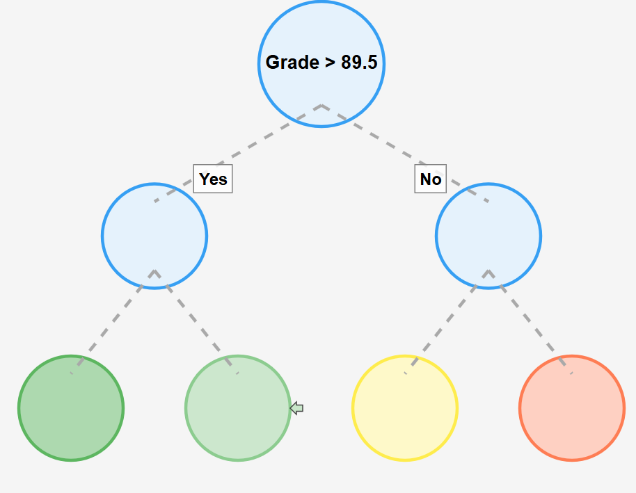
Suppose the best split is at θ = 89.5, with minimum Gini = 0.1

Then, the feature Average_Grade is represented by the binary rule :

Average_Grade ≤ 89.5

Final Decision for Root Node

Suppose we have Gini scores for all features :

• Degree_Type → Best Gini = 0.2667

• Average_Grade → Best Gini = 0.1

• Field → Still being evaluated

Choose the feature with lowest Gini impurity as the root node.

In this case : Average_Grade

Recursive Tree Building

• The tree recursively continues splitting based on feature thresholds .

• Splitting stops when :

  • Nodes are pure (Gini = 0), or

  • No further gain in Gini can be made.

Understanding Gini Impurity

Gini Impurity is a measure of how often a randomly chosen element from a dataset would be incorrectly classified if it were randomly labeled according to the distribution of labels in the subset.

The formula for Gini Impurity is :

Where :

• K = number of classes

• Pᵢ = probability of class i

Intuitive Example : Fruit in a Bag

Imagine a bag containing :

• 3 Oranges : O₁ , O₂ , O₃

• 2 Apples : A₁ , A₂ 

So, we have a total of 5 fruits.

Now, suppose you are blindfolded and asked to guess the fruit by picking one at random. If you guess “orange” every time, you’ll sometimes be correct (if it's actually an orange), and sometimes wrong (if it's an apple). The chance of being wrong represents the Gini impurity .

Pure Case: No Impurity

If the bag had only oranges (5 oranges) :

• Then any guess of “orange” is always correct.

• There is no uncertainty, and hence Gini impurity is 0.

This is a pure node — no impurity .

Mixed Case : Impure Node

Now, let’s revisit the original mix :

• 3 Oranges → P(O) = 3/5

• 2 Apples → P(A) = 2/5

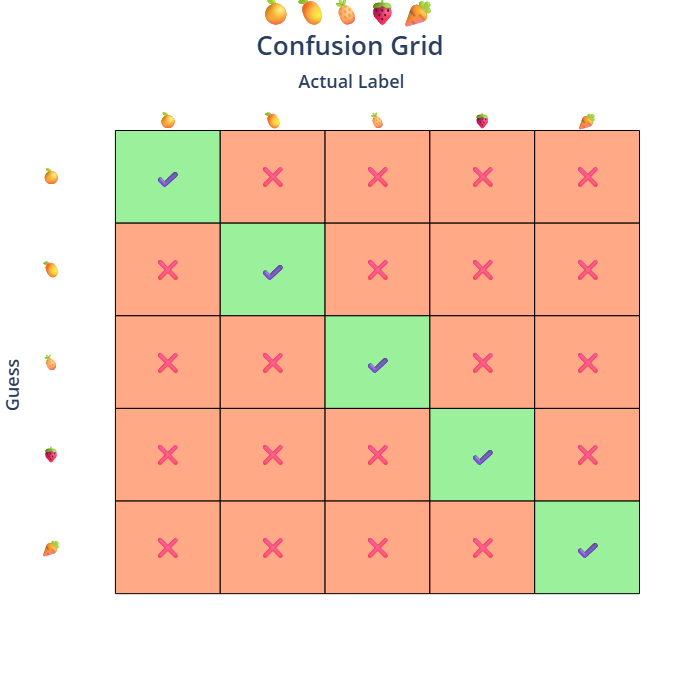
We can think of this scenario using a grid of guesses vs actuals :

• Horizontally : guessed labels

• Vertically : actual labels

• Highlight correct guesses in green and wrong guesses in red

Now, to compute the probability of wrong guesses, we subtract the correct guess probability from 1 :

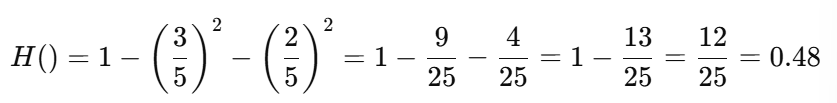
So, the Gini impurity is 0.48, indicating a fair level of impurity due to mixed classes .

Interpretation

• High Gini Impurity (~0.5) → Classes are mixed → High chance of wrong classification

• Low Gini Impurity (~0) → Classes are pure → Low or no chance of error

Why It Matters in Decision Trees

During splitting :

• The goal is to reduce Gini impurity as much as possible.

• At each step, we pick the split that leads to the lowest overall Gini.

• Pure nodes (Gini = 0) are ideal leaf nodes where no further splitting is needed.

More Variety, More Impurity

The more class labels we have in a dataset — each with equal probability — the higher the Gini impurity. This is because it becomes more difficult to make a correct guess consistently when there are many equally likely options .

Example: Maximum Variety Scenario

Suppose we have a bag containing 5 different items, each from a unique class:

• Orange

• Mango

• Guava

• Berry

• Carrot

Each class appears exactly once, so :

Gini Impurity Calculation

Interpretation

• The Gini impurity is 0.8, which is very high.

• This represents a high degree of uncertainty, as each class is equally likely and there's no dominant class.

Takeaway

• More distinct classes → Higher impurity

• Balanced class probabilities → Maximum impurity

• Gini impurity is lowest (0) when all elements belong to one class.

• Gini impurity is highest when the classes are equally distributed and numerous.

Pure Class Scenario: Zero Gini Impurity

Let’s now consider the case where all items in the dataset belong to one class.

Example : All Oranges

Suppose the bag contains:

• 5 Oranges

• No other fruit

Then, the probability of orange is :

P(Orange) = 5/5 = 1

All other classes : 0 .

Gini Impurity Calculation

Result

• The Gini impurity is 0, which means this node is pure.

• There is no uncertainty, and hence no chance of misclassification.

General Characteristics of Gini Impurity

• The range of Gini impurity is :

• Gini = 0 → Pure node (all elements from one class)

• Higher Gini → More class mixture, higher chance of wrong prediction

Goal in Decision Trees

• The goal of decision trees is to split the data in a way that:

  • Similar (or same-class) instances go to one side

  • Dissimilar instances go to the other

• Each split aims to reduce Gini impurity, ideally moving toward 0.

• When a leaf node is reached with Gini = 0, we stop — the node is pure, and further splitting is unnecessary.

Intuition

Classification is about organizing the system:

• Group similar items together

• Separate different items apart

• This “ordering” process minimizes impurity and improves classification accuracy

Geometric Intuition of Decision Trees

Let’s understand how a decision tree visually splits the data in feature space.

Suppose We Have the Following Features :

CGPA	IQ	Placement
—	—	Yes
—	—	No
—	—	—

We plot this data on a 2D plane where:

• X-axis : CGPA

• Y-axis : IQ

• Points are colored or marked based on placement (Yes/No)

How the Decision Tree Splits

First Split : Based on IQ > 80

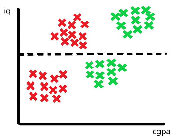
The decision tree considers all features and picks the best one to split on — say, IQ > 80 is chosen first.

• We draw a horizontal line at IQ = 80 on the graph.

• The data is now divided into two regions:

  • Above the line → IQ > 80

  • Below the line → IQ ≤ 80

• These regions correspond to different placement outcomes.

Second Split : Based on CGPA > 8 (in the IQ > 80 region)

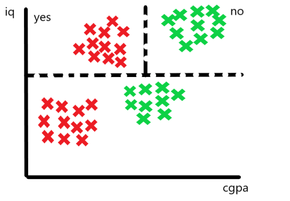
• We now examine the upper region (IQ > 80), and further split based on CGPA > 8.

• This results in vertical cuts in that sub-region of the data.

Another Split : Based on CGPA < 5 (in the IQ ≤ 80 region)

• Similarly, the tree now looks at the lower region (IQ ≤ 80) and splits based on CGPA < 5.

• If CGPA < 5, we may predict “Not Placed”; otherwise, “Placed”.

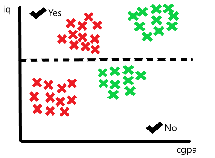
What’s Happening Visually

Each split creates an axis-aligned cut (either horizontal or vertical) in the feature space. These cuts continue recursively, resulting in a partitioning of the space into rectangular regions.

Each final region (leaf node) corresponds to a class label, assigned based on the majority class in that region.

Color-Coding Regions

• Points falling in the green region may be labeled “Placed”

• Points in the red region may be labeled “Not Placed”

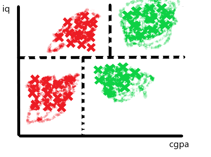
These regions are formed by a series of decisions that cut along the feature axes.

Higher Dimensions ?

In higher dimensions (more than 2 features), the decision tree still makes axis-aligned cuts, but instead of drawing lines, it creates hyperplanes (e.g., planes in 3D).

The idea remains the same:

• Split the space into purer and purer subsets

• Assign labels based on the dominant class in each subset

Final Insight

A decision tree divides the feature space into regions, and each region has a class label.

When a new data point arrives, we simply check which region it falls into — and assign the corresponding label.