
PCA (Principal Component Analysis)
- Aryan

- Mar 26, 2025
- 14 min read
CURSE OF DIMENSIONALITY
In machine learning, datasets consist of multiple columns, which are referred to as features. Features represent different attributes of the data and collectively define the dimensionality of the dataset. However, increasing the number of features beyond an optimal threshold can lead to performance degradation rather than improvement. This phenomenon is known as the curse of dimensionality.
Impact of High Dimensionality
When the number of features is excessively high, the model becomes computationally expensive, leading to a decline in performance. This happens because:
The model requires more computational resources.
Additional features may introduce noise rather than useful information.
The dataset becomes sparse, making it difficult to generalize well.
Example: Handwritten Digit Classification
Consider a handwritten digit classification problem, such as the MNIST dataset. Each digit image is of size 28×28 pixels, totaling 784 pixels per image. Each pixel is treated as a feature.
Some pixels contain valuable information about the digit, while others (such as background pixels) do not contribute much.
If we include all pixels as features, it may negatively impact the model by increasing computational complexity and reducing performance.
However, selecting only the most relevant pixels (features) improves model efficiency and accuracy.
This illustrates the curse of dimensionality, where increasing dimensions lead to computational inefficiency and performance issues.
The Role of Sparsity in High-Dimensional Space
As dimensionality increases, data points become sparsely distributed. This sparsity causes:
Difficulty in locating and clustering data points efficiently.
Increased computational time for distance-based models (e.g., K-Nearest Neighbors).
Reduced model effectiveness due to the lack of meaningful structure in high-dimensional space.
Solutions: Dimensionality Reduction
To address the curse of dimensionality, we use dimensionality reduction techniques, which reduce the number of features while retaining essential information. These techniques fall into two main categories:
Feature Selection
Selects a subset of the most relevant features from the original dataset.
Common methods include:
Forward Selection: Iteratively adds the best-performing features.
Backward Elimination: Iteratively removes the least important features.
Feature Extraction
Creates a new set of features by transforming existing features.
New features are often linear combinations of the original ones.
Popular techniques include:
Principal Component Analysis (PCA)
Linear Discriminant Analysis (LDA)
t-Distributed Stochastic Neighbor Embedding (t-SNE)
By applying dimensionality reduction, we optimize model performance, reduce computational costs, and mitigate the effects of high-dimensional sparsity.
Introduction to PCA and Its Purpose
Principal Component Analysis (PCA) is a feature extraction technique aimed at reducing the number of features (dimensions) in a dataset while preserving the essential information. By lowering the dimensionality, PCA helps improve the performance of machine learning models.
To understand how PCA works, consider an analogy:
Analogy: The Photographer’s Perspective
Imagine a photographer capturing images of a soccer match in a three-dimensional (3D) stadium. The goal is to publish these images in a newspaper, which can only display two-dimensional (2D) images. The photographer moves around the stadium to find the best angles that effectively represent the game’s dynamics.
Similarly, PCA projects high-dimensional data into a lower-dimensional space while retaining its most important characteristics. Just as the photographer selects the best perspective to capture meaningful photos, PCA selects the most informative axes that best describe the data’s variability.
GEOMETRIC INTUITION OF PCA
Example: House Dataset
Suppose we have a dataset of houses with three columns:
Number of rooms – Represents how many rooms are in a house.
Number of grocery shops nearby – Indicates the count of nearby grocery stores.
Price (in lakhs) – The price of the house in lakhs.
No. of rooms | No. of grocery shops | Price(L) |
3 | 2 | 60 |
4 | 0 | 130 |
5 | 6 | 170 |
2 | 10 | 90 |
In this dataset, the number of grocery shops is given, but we assume it is not a significant feature, meaning it does not strongly impact the house price.
Understanding Feature Selection
Feature selection is the process of choosing the most relevant features from a dataset. Instead of using all available columns, we select only those that have a significant impact on the target variable (in this case, price). For example, if we have five features, we may select only two or three that contribute the most to our prediction model.
In our given dataset, we have two input columns: Number of rooms and Number of grocery shops nearby. Since the number of rooms is likely a more important factor in determining house price than the number of grocery shops, we can remove the grocery shops column.
Thus, we keep only the Number of rooms column, as it has a stronger influence on the price of the house. In this case, it is easy to determine that the number of rooms is a more significant predictor of price than the number of grocery shops nearby.
As machine learning engineers, we often work with different types of datasets, some of which we may not have domain knowledge about. In such cases, we may be unsure about which features to select. Let's discuss a mathematical trick to help with feature selection.
We plotted the given data in a two-dimensional coordinate space.
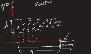
From the plot, we observe that the number of rooms varies significantly, whereas the number of grocery shops nearby does not change as much. Additionally, there is no strong direct relationship between the two features.
Whenever we encounter such data in a scatter plot, we should examine the spread of our data along each axis. The key idea is to determine which feature has a higher variance (spread).
Let d be the length of projection on the x-axis (representing the number of rooms).
Let d' be the length of projection on the y-axis (representing the number of grocery shops).
If d > d', it means that the number of rooms has a higher spread than the number of grocery shops. By simply observing this, we can conclude that the number of rooms is a more important feature than the number of grocery shops .
Key Takeaway
We select features that have higher variance (greater spread) because they provide more useful information for modeling. In this case, since the number of rooms exhibits more variation than the number of grocery shops nearby, we choose rooms as the more relevant feature.
Understanding Feature Extraction
In the previous example, we solved the problem using feature selection. However, there are cases where feature selection alone is not sufficient.
Let's consider a new scenario where our dataset changes. Instead of the number of grocery shops, we now have the number of washrooms as a feature :
No. of rooms | No. of Washrooms | Price (L) |
Now, if we need to select one input feature, we face a challenge. In this scenario, both input features are important, and we are uncertain which one to choose. The price depends equally on both the number of rooms and the number of washrooms, making it difficult to decide which feature to retain. Feature selection is not as useful in this case.
To analyze this, we plot the data :

From the graph, we observe a linear relationship between the number of rooms and the number of washrooms. As the number of rooms increases, the number of washrooms also increases.
If we project the data onto the x-axis (rooms) and call the spread d, and onto the y-axis (washrooms) and call the spread d', we find that d ≈ d'. This means the two features have almost equal variance .
Why Feature Selection Fails
When two features have nearly the same variance and are highly correlated, selecting one over the other becomes mathematically difficult. In such cases, we cannot simply remove one feature based on variance alone.
Solution: Feature Extraction
Instead of removing a feature, we can apply feature extraction techniques such as Principal Component Analysis (PCA) to transform the data into a new feature space. Feature extraction helps combine multiple correlated features into a new set of independent features, retaining essential information while reducing redundancy.
Thus, when variance alone is not enough to decide which feature to keep, feature extraction provides a better approach to handle the data efficiently .
Understanding PCA and Feature Extraction
In our dataset, we have rooms, washrooms, and price as features. The challenge is to remove one of the input columns (rooms or washrooms).
If we consult a domain expert, they might suggest a different way to structure the data. Instead of selecting either rooms or washrooms, they might suggest using flat size as a new feature because a larger flat generally has more rooms and washrooms. This means we replace the original features with a new, more meaningful one.
Similarly, Principal Component Analysis (PCA) works in a way where it forgets existing features and creates a new set of features (principal components) by selecting subsets of features with the highest variance. But what if we do not have domain knowledge? In that case, PCA helps us decide.
What Does PCA Do in This Scenario?
PCA finds a new set of coordinate axes by rotating the data to align with the directions of maximum variance.
PCA rotates the coordinate axes to form a new set of axes.
In this new coordinate system, we measure the spread (variance) along the new axes.
Suppose the new "rooms'" axis has variance d, and the new "washrooms'" axis has variance d'. If d > d', then we select the "rooms'" axis and discard the "washrooms'" axis.
These new axes are called Principal Component 1 (PC1) and Principal Component 2 (PC2).
The principal component with the highest variance is selected, and the data is transformed accordingly .
How Many Principal Components Do We Get?
The number of principal components (PCs) is always less than or equal to the number of original features:
No. of PCs ≤ No. of original features (n)
PCA essentially reorients the data along new axes where the spread is maximized. This helps in reducing redundancy and improving efficiency in feature representation.
By applying PCA, we can reduce dimensionality while retaining the most informative aspects of the data, making it a powerful tool for feature extraction in cases where domain knowledge is lacking .
Benefits of PCA
PCA offers several advantages, particularly in data analysis and machine learning:
Dimensionality Reduction: By reducing the number of features, PCA makes computations faster and avoids overfitting in models.
Noise Reduction: By retaining only the most important components, PCA filters out noise and irrelevant variations in the data.
Improved Visualization: Humans can only perceive up to three dimensions; PCA enables complex, high-dimensional data to be transformed into 2D or 3D representations, facilitating better understanding and analysis.
Feature Extraction: Unlike feature selection, PCA creates new, transformed features that capture the most significant information in the dataset .
Importance of Variance in PCA
In Principal Component Analysis (PCA), variance plays a crucial role in how the algorithm functions and why it's effective for dimensionality reduction. Here's a breakdown of its importance:
Core Concept:
Maximizing Variance:
PCA aims to find new axes (principal components) that capture the maximum variance in the data. In essence, it seeks directions in which the data points are most spread out.
This is because higher variance generally indicates that the data contains more information along that direction.
Why Variance Matters:
Information Retention:
By prioritizing principal components with high variance, PCA ensures that the most significant patterns and relationships within the data are preserved.
Conversely, components with low variance contribute less information and can often be discarded without substantial loss of data integrity.
Dimensionality Reduction:
The goal of PCA is to reduce the number of variables (dimensions) while retaining as much essential information as possible.
By selecting only the principal components that explain a large portion of the total variance, we can effectively compress the data without sacrificing its key characteristics.
Identifying Important Features:
The amount of variance explained by each principal component provides a measure of its importance.
This allows us to identify which features or combinations of features contribute most significantly to the overall variability of the data.
Explained Variance:
"Explained variance" is a metric that quantifies the proportion of the total variance in the original data that is captured by each principal component.
This metric is vital for determining the optimal number of principal components to retain.
In simpler terms :
Imagine your data as a cloud of points in space. PCA tries to find the "directions" where the cloud is most spread out. These directions are the principal components. The more spread out the cloud is in a direction (higher variance), the more "information" that direction holds.
Therefore, variance is the key to PCA's ability to simplify complex data while preserving its essential structure .

Projecting a 2D Dataset to 1D
Suppose we have a 2D dataset, and we need to reduce it to 1D. The dataset transformation can be visualized as shown in the image above.

Let's consider a single point in a 2D space. This point has coordinates (x,y) along the x-axis and y-axis. We can represent this point as a vector x, which has two components:
x-component
y-component
Since we aim to reduce the dimensionality, we must project this vector onto another vector. The goal is to find the unit vector in a particular direction and project x onto it .
Finding the Unit Vector and Projection

Choosing the Optimal Unit Vector
Since our goal is to maximize variance, the question arises: Which unit vector should we choose?
The optimal unit vector is the one that results in the maximum variance of the projected points.
To understand how variance is calculated, consider a vector x and a unit vector u. When we project x onto u, the projection is computed using the formula discussed in the previous section.
The formula for variance is :

Now, transforming this equation for the projection onto u, we get :

This expression represents the variance of the projected data along the unit vector u .
Principal Component Analysis (PCA)
In PCA, the objective is to find the unit vector u such that when all points are projected onto it, the variance is maximized. This means we seek the unit vector u that maximizes :

Covariance and Covariance Matrix
Covariance measures how two variables change together. If an increase in one variable corresponds to an increase in another, the covariance is positive; if an increase in one corresponds to a decrease in the other, it's negative.
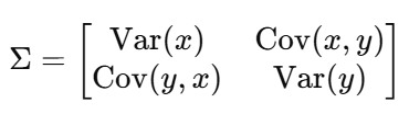
The covariance matrix is a square matrix that summarizes the covariances between multiple variables in a dataset.
For 2D data (x, y), the covariance matrix is :
For 3D data (x, y, z), the covariance matrix extends to :

Key Properties :
The covariance matrix is symmetric.
Diagonal elements represent variances.
Off-diagonal elements represent covariances.
Benefits of Covariance Matrix
It helps understand how different features are correlated.
Used in Principal Component Analysis (PCA) for dimensionality reduction.
Plays a role in multivariate statistical analysis and Gaussian distributions.
Linear Transformations and Matrices
A linear transformation maps a vector space to another while preserving vector addition and scalar multiplication.
Matrices perform linear transformations by rotating, scaling, or shearing data.
Example: Scaling transformation using matrix multiplication

scales the x-axis by 2 and the y-axis by 3.
Eigenvalues, Eigenvectors, and Eigen Decomposition
Eigenvectors are special vectors whose direction remains unchanged when a linear transformation is applied.
Eigenvalues represent the factor by which the eigenvector is stretched.
If A is a matrix and v is an eigenvector, then:
Av = λv
where λ is the eigenvalue.
Eigen decomposition of a matrix A :

where :
Q is a matrix of eigenvectors,
Λ is a diagonal matrix of eigenvalues.
Application in PCA :
The eigenvectors of the covariance matrix give the principal components.
Eigenvalues indicate how much variance each principal component captures.
By selecting the top k eigenvectors, we reduce dimensionality while preserving maximum variance .
Eigen Decomposition of the Covariance Matrix
To find the optimal unit vector u, we consider the covariance matrix of the data. The covariance matrix Σ captures the spread of data across different dimensions.
The key idea in PCA is that the eigenvectors of the covariance matrix represent the principal directions of variation in the data. The corresponding eigenvalues indicate the amount of variance along these directions.
The largest eigenvector (corresponding to the largest eigenvalue) is the principal component that captures the maximum variance.
The unit vector u that maximizes variance is precisely this eigenvector.
Thus, the first principal component is the eigenvector associated with the largest eigenvalue of the covariance matrix Σ , and it provides the best low-dimensional representation of the data in terms of variance.
Largest Eigenvector :
The eigenvector corresponding to the largest eigenvalue of the covariance matrix points in the direction of the greatest variance (spread) in the data. The magnitude of this eigenvector is equal to the corresponding eigenvalue, which quantifies the variance in that direction.
Second Largest Eigenvector :
The eigenvector associated with the second largest eigenvalue is orthogonal (perpendicular) to the largest eigenvector. It points in the direction of the second greatest variance in the data, capturing the next most significant spread.
Key Insight :
Eigenvectors of the covariance matrix identify the principal directions of data spread :
The largest eigenvector represents the primary direction of variance.
Subsequent eigenvectors (which are mutually orthogonal) represent directions of decreasing variance.
These eigenvectors form the basis for Principal Component Analysis (PCA), which reduces dimensionality while preserving maximum variance.
Step-by-Step Explanation of How PCA Solves the Problem
Principal Component Analysis (PCA) is a technique used to reduce the dimensionality of data while preserving as much variance as possible. Below is a step-by-step breakdown of how PCA works :
Mean Centering the Data
First, we compute the mean of each feature (column) and subtract it from the corresponding data points.
This ensures that the dataset is centered around the origin, making it easier to analyze its variance.
Computing the Covariance Matrix
The covariance matrix captures relationships between different variables in the dataset.
It helps us understand how changes in one variable affect others.
Finding Eigenvalues and Eigenvectors
We compute the eigenvalues and eigenvectors of the covariance matrix.
Eigenvectors represent the principal directions (principal components) of the data, while eigenvalues indicate the amount of variance in those directions.
We obtain three eigenvectors (for three input features) and their corresponding eigenvalues.
Selecting Principal Components
The eigenvector with the highest eigenvalue represents the direction of maximum variance and is selected as the first principal component (PC1).
If we need further dimensionality reduction, we can take the second principal component (PC2) and so on.
We can choose to reduce the data from 3D to 2D (using PC1 and PC2) or from 3D to 1D (using only PC1).
Projecting Data onto Principal Components
Finally, we transform the original dataset by projecting it onto the selected principal components.
This reduces the dimensionality while retaining the most important patterns in the data.
Transforming Points Using PCA
After identifying the principal components, we need to transform our data from a higher-dimensional space to a lower-dimensional space using a dot product operation. Below is a step-by-step explanation:
Understanding the Data Shape Before Transformation
Suppose our dataset consists of three features (f1, f2, f3) and one target variable.
Initially, the dataset is in 3D with a shape of (1000,3) (1000 data points with 3 features).
If we reduce it to 1D, it becomes (1000,1); if reduced to 2D, it becomes (1000,2).
Projecting Data onto Principal Components
To transform the data, we project all points onto the selected principal component (e.g., PC1).
This is done using the dot product of the principal component vector u and the data points x.
Computing the Dot Product
The shape of our original data is (1000,3).
The principal component uuuis a (1,3) vector (since it has three dimensions).
We first transform u into a (3,1) vector to match the dimensions for matrix multiplication.
Performing the Matrix Multiplication
The dot product of (1000,3) × (3,1) results in a transformed dataset of shape (1000,1).
If projecting onto two principal components (PC1 and PC2), we perform a similar operation, resulting in (1000,2).
FINDING OPTIMUM NUMBER OF PRINCIPAL COMPONENTS
When we apply PCA to a dataset with high dimensionality (e.g., 784 features), we get 784 principal components, each associated with an eigenvalue :

Each eigenvalue (λ) represents the amount of variance captured by its corresponding principal component. The larger the eigenvalue, the more variance that component explains .
Step to Calculate Percentage Variance Explained

Choosing the Optimal Number of Components
Our goal is to retain most of the data’s information (usually 90% or more of total variance).
To do this, sum the eigenvalues cumulatively and find the number of components needed to reach 90% of the total variance .
Example
Suppose the eigenvalues are :

If the sum of the first 15 eigenvalues accounts for over 90% of the total variance, then: We can safely reduce the data to 15 dimensions using the first 15 principal components.
To determine the optimal number of components:
Apply PCA and get eigenvalues.
Convert eigenvalues to percentage of explained variance.
Cumulatively sum them.
Choose the smallest number of components that together explain ≥ 90% of total variance .
WHEN PCA DOES NOT WORK

Principal Component Analysis (PCA) is a powerful dimensionality reduction technique, but it has limitations :
Distribution :
If the data distribution is circular (as shown in the first diagram), the variance along both the x and y axes is equal in certain scenarios .
Since PCA relies on finding the directions of maximum variance, it does not provide meaningful dimensionality reduction in this case. No matter how we rotate the axes or compute the eigenvectors, the variance remains the same in all directions, making PCA ineffective.
Higher-Dimensional Data with No Clear Alignment :
If the data exists in a higher-dimensional space but lacks a clear alignment or direction of variance, applying PCA does not yield significant benefits. PCA works best when the data exhibits strong correlations along certain directions.
Non-Linear Patterns :
If the data follows a structured but non-linear pattern (as seen in the third diagram), reducing the dimensionality using PCA can lead to the loss of important information. Since PCA is a linear transformation, it cannot effectively capture complex structures such as curved or clustered patterns.
In such cases, alternative techniques like kernel PCA, t-SNE, or autoencoders might be more suitable for dimensionality reduction.


