LOGISTIC REGRESSION - 4

MLE IN MACHINE LEARNING

In any dataset where the distribution is known, we can use Maximum Likelihood Estimation (MLE) to determine the parameters of that distribution.

Given a set of data points, we first assume a specific distribution. We then construct a likelihood function and find the parameter values that maximize this function. This process can be broken down into three steps.

Now, the question arises : how can we apply this flow in machine learning ?

In machine learning, we work with training data, which consists of input features ( x₁ , x₂ , x₃ , ..., xₙ) and an output variable (y). If (y) has two classes, such as "yes" and "no," it follows a Bernoulli distribution. If (y) has multiple classes, it follows a multinomial or multinoulli distribution.

The process of applying Maximum Likelihood Estimation in machine learning can be outlined in the following steps :

1. Identify the Distribution : We first aim to determine the distribution of (y) given (x), denoted as ( P(y | x) ).

2. Select a Model : Based on the identified distribution, we choose a parametric machine learning model. MLE techniques are applicable only to models that are parametric in nature.

3. Initialize Parameters : We randomly assign initial values to our model parameters.

4. Choose a Likelihood Function : We select a likelihood function that corresponds to the distribution of the data.

5. Optimize Parameters : We then find the parameter values that maximize the likelihood function. At this point, our model is considered trained.

we have utilized the concept of Maximum Likelihood Estimation to train our model. This means that if we have a parametric function, we can train our model using MLE to find the parameter values that yield the maximum likelihood.

MLE IN LOGISTIC REGRESSION

We have four training points and two models. The question is: Which model is best ?

The answer is : Model 1 is better because it is able to separate red and green points onto different sides of the decision boundary. Model 2 fails to do this.

Now, if we have two models like this :

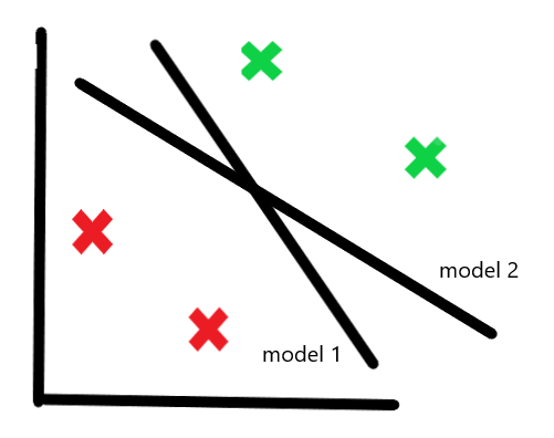
How do we choose between them ?

Both models correctly classify all points, so how do we differentiate which one is better ?

We can use the sigmoid function on each point to calculate the probability of that point being green. Once we have the probabilities for all points, we multiply the probabilities of the actual outcomes :

• Probability of green points being predicted as green

• Probability of red points being predicted as red

This concept is known as Maximum Likelihood Estimation (MLE).

We take the probability of the actual class :

• For green points → probability of being predicted as green

• For red points → probability of being predicted as red

We calculate the MLE for each line. The line with the highest MLE is considered the best.

MLE Derivation : Step-by-Step

Suppose we have data like x₁ , x₂ , x₃ , ... ∣ y

There are n input columns and one output column.

We first need to understand what the output depends on : it clearly depends on the input features x . So, we write this relationship as :

                                y ∣ x

Step 1 : Assume a Distribution for the Output (y)

In logistic regression, this step is straightforward.

Since the output column consists of 0s and 1s (binary classification), the natural choice is the Bernoulli distribution.

You might wonder — why not a Binomial distribution?

Here’s the reason :

• Each row in the dataset represents a single observation or query point

• Each prediction is made independently

• Each output can only take two values : 0 or 1

While it may look like a binomial distribution because we have many rows, the actual prediction happens one point at a time. So each output is best modeled using the Bernoulli distribution.

However, if we were asked : How many 1s are predicted out of 100 points ? — then we’d use the Binomial distribution.

Summary :

We assume that the output variable y follows a Bernoulli distribution in logistic regression.

Step 2 : Choose a Parametric Model

We choose a parametric machine learning model — specifically, Logistic Regression.

This means that the relationship between x and y is modeled using a function (sigmoid), and the function depends on parameters (the coefficients). These parameters will be learned using the MLE method.

Step 3 : Initialize Coefficients

We randomly choose the initial values for the coefficients (also called model parameters). This gives us a starting point for optimization.

Step 4 : Assume a Likelihood Function

We need to assume a likelihood function based on the distribution of the output variable y . Since y is binary (0 or 1), we assume it follows a Bernoulli distribution.

So, for a single data point :

Where :

• P is the predicted probability of y = 1

• 1 − p is the predicted probability of y = 0

• k ∈ {0,1} is the actual observed value from the output column

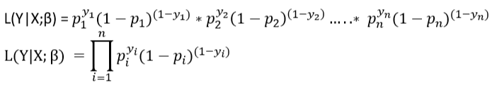
Likelihood Function for Multiple Data Points

Let us define the likelihood of y given x , parameterized by β :

                                                L ( Y | X ; β )

Assume all data points are independent. Then, for n data points :

For mathematical convenience, we transform the Bernoulli probability mass function (PMF) from :

                                    pk + (1−p) (1−k)

to the equivalent exponential form :

This transformation is helpful because both expressions give the same result, but the exponential form simplifies the process of taking the logarithm, which we need for optimization.

Now we take the logarithm of both sides of the likelihood function :

We break this product into two parts using logarithmic properties :

Applying the power rule of logarithms :

This is our log-likelihood function

We have to maximize this term , we want that values of coefficients for which this will give maximum value , we can apply gradient descent technique to find that values of coefficients.We aim to maximize this log-likelihood function. In other words, we want to find the values of the model coefficients (parameters) that maximize this expression. To achieve this, we can apply an optimization technique such as gradient descent, which iteratively adjusts the coefficients to reach the point where the log-likelihood is at its maximum.

SOME IMPORTANT QUESTIONS

1. Is MLE a general concept applicable to all machine learning algorithms ?

   - Maximum Likelihood Estimation (MLE) is a general statistical concept that can be applied to many machine learning algorithms, particularly those that are parametric (i.e., defined by a set of parameters), but it’s not applicable to all machine learning algorithms. MLE is commonly used in algorithms such as linear regression, logistic regression, and neural networks to find the optimal values of the parameters that best fit the training data. However, some machine learning algorithms don’t rely on MLE. For example :

     1. Non-parametric methods : Some machine learning methods, such as k-Nearest Neighbors (k-NN) and Decision Trees, are non-parametric and do not make strong assumptions about the underlying data distribution. These methods don’t have a fixed set of parameters that can be optimized using MLE.

     2. Unsupervised learning algorithms : Some unsupervised learning algorithms, like K-means clustering, use different objective functions, not necessarily tied to a probability distribution.

     3. Reinforcement Learning : Reinforcement Learning methods generally don’t use MLE, as they are more focused on learning from rewards and punishments over a sequence of actions rather than fitting to a specific data distribution.

2. How is MLE related to the concept of loss functions ?

   - In machine learning, a loss function measures how well a model's predictions align with the actual values. The goal of training a machine learning model is often to find the model parameters that minimize the loss function. Maximum Likelihood Estimation (MLE) is a method of estimating the parameters of a statistical model to maximize the likelihood function, which is conceptually similar to minimizing a loss function. In fact, for many common models, minimizing the loss function is equivalent to maximizing the likelihood function. MLE and the concept of loss functions in machine learning are closely related. Many common loss functions can be derived from the principle of maximum likelihood estimation under certain assumptions about the data or the model. By minimizing these loss functions, we’re effectively performing maximum likelihood estimation.

3. Then why does loss function exist, why don't we maximize likelihood ?

   - The confusion arises from the fact that we’re using two different perspectives to look at the same problem. In many machine learning algorithms, the aim is to minimize the difference between the predicted and actual values, and this is typically represented by a loss function. When we talk about minimizing the loss function, it’s essentially the same as saying we’re trying to find the best model parameters that give us the closest predictions to the actual values. On the other hand, when we look at the problem from a statistical perspective, we talk in terms of maximizing the likelihood of seeing the observed data given the model parameters. This is represented by a likelihood function. For many models, these two perspectives are equivalent - minimizing the loss function is the same as maximizing the likelihood function. In fact, many common loss functions can be derived from the principle of MLE under certain assumptions about the data. So why do we often talk about minimizing the loss function instead of maximizing the likelihood ? There are a few reasons :

     1. Computational reasons : It’s often easier and more computationally efficient to minimize a loss function than to maximize a likelihood function. This is particularly true when working with complex models like neural networks.

     2. Generalization : The concept of a loss function is more general and can be applied to a wider range of problems. Not all machine learning problems can be framed in terms of maximizing a likelihood. For example, many non-parametric methods and unsupervised learning algorithms don’t involve likelihood.

     3. Flexibility : Loss functions can be easily customized to the specific needs of a problem. For instance, we might want to give more weight to certain types of errors, or we might want to use a loss function that is robust to outliers.

4. Then why study about maximum likelihood at all ?

   - The study of Maximum Likelihood Estimation (MLE) is essential for several reasons, despite the prevalence of loss functions in machine learning :

     1. Statistical Foundation : MLE provides a strong statistical foundation for understanding machine learning models. It gives a principled way of deriving the loss functions used in many common machine learning algorithms, and it helps us understand why these loss functions work and under what assumptions.

     2. Interpretability : The MLE framework gives us a way to interpret our model parameters. The MLEs are the parameters that make the observed data most likely under our model, which can be a powerful way of understanding what our model has learned.

     3. Model Comparison : MLE gives us a way to compare different models on the same dataset. This can be done using tools like the Akaike Information Criterion (AIC) or the Bayesian Information Criterion (BIC), which are based on the likelihood function and can help us choose the best model for our data.

     4. Generalization to Other Methods : MLE is a specific case of more general methods, like Expectation-Maximization and Bayesian inference, which are used in more complex statistical modeling. Understanding MLE can provide a stepping stone to these more advanced topics.

     5. Deeper Understanding : Lastly, understanding MLE can give us a deeper understanding of our models, leading to better intuition, better model selection, and ultimately, better performance on our machine learning tasks. In short, while you can often get by with a practical understanding of loss functions and optimization algorithms in applied machine learning, understanding MLE can be extremely valuable for gaining a deeper understanding of how and why these models work.

In short, while you can often get by with a practical understanding of loss functions and optimization algorithms in applied machine learning, understanding MLE can be extremely valuable for gaining a deeper understanding of how and why these models work.

Assumptions of Logistic Regression

Logistic regression, like other statistical methods, relies on certain assumptions. Here are the main assumptions of logistic regression :

1. Binary Logistic Regression requires the dependent variable to be binary :

   That means the outcome variable must have two possible outcomes, such as "yes" vs "no", "success" vs "failure", "spam" vs "not spam", etc.

   
   

2. Independence of observations :

   The observations should be independent of each other. In other words, the outcome of one instance should not affect the outcome of another.

   
   

3. Linearity of independent variables and log odds :

   Although logistic regression does not require the dependent and independent variables to be related linearly, it requires that the independent variables are linearly related to the log odds.

   
   

4. Absence of multicollinearity :

   The independent variables should not be too highly correlated with each other, a condition known as multicollinearity. While not a strict assumption, multicollinearity can be a problem because it can make the model unstable and difficult to interpret.

   
   

5. Large sample size :

   Logistic regression requires a large sample size. A general guideline is that you need at least 10 cases with the least frequent outcome for each independent variable.

   For example, if you have 5 independent variables and the expected probability of your least frequent outcome is 0.10, then you would need a minimum sample size of :

   500 = (10 × 5) / 0.10

Note : That violating these assumptions doesn't mean you can't or shouldn't use logistic regression, but it may impact the validity of the results and you should proceed with caution.

Odds and log(odds)

Odds :

The odds of an event is the ratio of the probability of the event happening (P) to the probability of the event not happening (1 - P). It's a way of expressing the likelihood of an event. If the odds are greater than 1, the event is more likely to happen than not, and vice versa.

Suppose you roll a die, and you are asked to find the odds of getting a 3.

1. Find the probability of getting a 3 :

   The probability of rolling a 3 on a fair die is P(3) = 1/6

2. Find the probability of not getting a 3 :

   The probability of not rolling a 3 is P (not 3) = 1 − P(3) = 5/6

3. Calculate the odds of getting a 3 :

   The odds are the ratio of the probability of success (getting a 3) to the probability of failure (not getting a 3). So, the odds are :

4. This means, "the odds of getting a 3 are 1 in 5 times."

General Formula for Odds :

In general, if p is the probability of success, the odds are given by the formula :

where p lies between 0 and 1, and the odds range from 0 to infinity.

log(Odds)

Sometimes, when dealing with odds, it can be difficult to interpret and compare them directly, especially when they vary widely. To address this, we take the logarithm of the odds, also known as log-odds, to make comparisons easier and to transform the scale into a more symmetric one.

1. Understanding the Concept of Odds :

   • Suppose we have a team that loses 1 match and wins 4 matches. The odds of winning for this team are :

     Odds of winning = 4/1 = 4

   • On the other hand, another team wins 1 match and loses 4. The odds of winning for this team are :

     Odds of winning = 1/4 = 0.25

2. Problem with Unevenness :

   • If we plot these odds on a number line :

     • The odds of the first team (4) would be a large value.

     • The odds of the second team (0.25) would be a small value.

   • This creates an asymmetry. The team with more wins has odds between 1 and infinity, while the team with more losses has odds between 0 and 1. Understanding and comparing these two on the same scale can be challenging.

3. Symmetry through Logarithms :

   • To make the scale symmetric and easier to compare, we take the logarithm of the odds.

   • Applying the logarithm to the odds :

     log (4) = 0.602

   log (0.25) = − 0.602

   • After applying the logarithm, the difference between the two values becomes smaller, and the scale becomes more symmetric. Now both values can be compared more easily.

Why Take Log(Odds) ?

• Taking the log of odds transforms the scale, making it symmetrical and easier to interpret. It helps overcome the challenge of comparing probabilities or odds that differ significantly.

• In practice, log-odds are often used in logistic regression to model probabilities, as they can take any real value, making them more useful for analysis.

Another interpretation of logistic regression

Understanding How Log(Odds) is Connected to Logistic Regression

In logistic regression, the relationship between probability and predictors is modeled using the log of the odds (log-odds) :

Dataset Example

Suppose we have a dataset that contains two input features — CGPA and IQ, and one output column called placement. The output column contains binary values : 1 for placed and 0 for not placed.

We apply logistic regression to this dataset for prediction.

Let Ŷ represent the predicted probability of getting placed, i.e., P(1) , which we denote as p (a small p).

cgpa	iq	placement	Ŷ (Predicted Probability)
8	80	1	0.93
-	-	0	0.37
-	-	0	0.21

Logistic Regression Formula

For the first student :

βX = 0 + (1)(8) + (2)(80) = 168

Now , we plug this into the sigmoid (logistic) function to calculate the probability of being placed :

Connecting to Log-Odds

We start with the sigmoid expression and manipulate it to derive the log-odds relation :

This means there is a linear relationship between the log of odds and the input features (X).

If we plot a graph of log(odds) vs X, the relationship should be linear :

Important Insight

It should be linear. If it is not linear, then our logistic regression model may not provide accurate results.

POLYNOMIAL FEATURES

Logistic regression essentially performs classification by drawing a linear decision boundary. However, if the classes in our dataset are not linearly separable, a simple linear boundary may not yield good accuracy.

The good news is that even though logistic regression is a linear model, we can still model non-linear decision boundaries by using polynomial features.

How It Works

Suppose we have one input feature x , and we want to capture non-linearity by transforming it using polynomial terms.

If we choose a polynomial degree of 2, then we transform our input feature into :

x⁰ , x¹ , x²

So instead of having just one input column, we now have three input columns.

Originally, we had parameters β₀ and β₁ , but after polynomial transformation, we now have :

β₀ , β₁ , β₂

This transformation allows the logistic regression model to fit non-linear decision boundaries, making it more flexible for complex data.

Important Consideration

• If we choose a very high polynomial degree, the model may overfit — it will fit the training data very well but perform poorly on unseen data.

• If we choose a very low degree, the model may underfit — it won't capture the complexity of the data.

Therefore, it's important to find an optimal polynomial degree — not too high and not too low — to balance bias and variance.

REGULARIZATION IN LOGISTIC REGRESSION

Regularization is a technique used in machine learning models to prevent overfitting, which occurs when a model learns the noise along with the underlying pattern in the training data. Overfitting leads to poor generalization performance when the model is exposed to unseen data.

In the context of linear models like linear regression and logistic regression, regularization works by adding a penalty term to the loss function that the model tries to minimize. This penalty term discourages the model from assigning too much importance to any single feature, which helps to prevent overfitting.

The most common types of regularization in linear models are L1 and L2 regularization :

1. L1 regularization (Lasso Regression) : This technique adds a penalty term equal to the absolute value of the magnitude of the coefficients. Mathematically, it's represented as the sum of the absolute values of the weights ( ‖w‖₁). This can lead to sparse models, where some feature weights can become exactly zero. This property makes L1 regularization useful for feature selection.

2. L2 regularization (Ridge Regression) : This technique adds a penalty term equal to the square of the magnitude of the coefficients. Mathematically, it's represented as the sum of the squared values of the weights ( ‖w‖₂² ​). L2 regularization tends to spread the weight values more evenly across features, leading to smaller, but non-zero, weights.

   
   

There's also Elastic Net regularization, which is a combination of L1 and L2 regularization. The contribution of each type can be controlled with a separate hyperparameter.

In all these techniques, the amount of regularization to apply is controlled by a hyperparameter, often denoted as λ (lambda). Higher values of λ mean more regularization, leading to simpler models that might underfit the data. Lower values of λ mean less regularization, leading to more complex models that might overfit the data. The optimal value of λ is typically found through cross-validation.