Multiple Linear Regression

Multiple Linear Regression is an extension of simple linear regression. Unlike simple linear regression, which involves one input feature (independent variable) and one output (dependent variable), multiple linear regression involves more than one input feature and still predicts a single output.

We use it when there are multiple predictors (input variables) influencing the target.

Example Dataset

Suppose we have data for 1000 students :

CGPA	IQ	Placement
8	80	8
9	90	9
5	120	15
...	...	...

In this case, we have two input features: CGPA and IQ, and one target variable: Placement.

Since we have multiple input columns, we use Multiple Linear Regression.

The model takes CGPA and IQ as inputs and predicts Placement.

Mathematical Equation

The equation of the regression line becomes :

y = β₀ + β₁x₁ + β₂x₂

where :

• x₁ -> CGPA

• x₂ -> IQ

• β₀ -> Intercept (bias term)

• β₁ , β₂ -> slopes (weights)

If we have n input features, the equation generalizes to :

y = β₀ + β₁x₁ + β₂x₂ + ⋯ + βₙxₙ

Geometric Interpretation

• In simple linear regression, the model fits a line in 2D space.

• In multiple linear regression with 2 features, it fits a plane in 3D space.

• In higher dimensions (n > 2), the model fits a hyperplane in n-dimensional space.

Objective of the Model

The goal of multiple linear regression is to find the optimal values of:

β₀ , β₁ , β₂ , … , βₙ​

These are the coefficients (weights) of the model.

The algorithm tries to fit a hyperplane that minimizes the error between the predicted and actual output. In other words, it tries to find a surface that is as close as possible to all data points in high-dimensional space.

Mathematical Formulation of Multiple Linear Regression

Let’s consider data from three students of a college. Our goal is to apply Multiple Linear Regression to predict placement based on CGPA and IQ.

Assume we know the coefficient values β₀ , β₁ , β₂ .

We want to predict:

ŷ₁ = ?    ŷ₂ = ?   ŷ₃ = ?

To calculate the predicted outputs (ŷᵢ):

ŷ₁ = β₀ + β₁.8 + β₂.80

ŷ₂ = β₀ + β₁.7 + β₂.70

ŷ₃ = β₀ + β₁.5 + β₂.120

Or more generally, using variable notation:

ŷ₁ = β₀ + β₁x₁₁ + β₂x₁₂

ŷ₂ = β₀ + β₁x₂₁ + β₂x₂₂

ŷ₃ = β₀ + β₁x₃₁ + β₂x₃₂

Now, suppose we have m input features and n students (i.e., n training samples).

Each prediction becomes:

ŷᵢ = β₀ + β₁xᵢ₁ + β₂xᵢ₂ + β₃xᵢ₃ + ⋯ + βₘxᵢₘ

So for all students:

ŷ₁ = β₀ + β₁x₁₁ + β₂x₁₂ + ⋯ + βₘx₁ₘ

ŷ₂ = β₀ + β₁x₂₁ + β₂x₂₂ + ⋯ + βₘx₂ₘ

ŷ₃ = β₀ + β₁x₃₁ + β₂x₃₂ + ⋯ + βₘx₃ₘ

⋮

ŷₙ = β₀ + β₁xₙ₁ + β₂xₙ₂ + ⋯ + βₘxₙₘ

Matrix Form (Compact Representation)

Let’s express all predictions in matrix form:

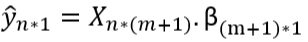
Prediction vector Ŷ :

Matrix Representation :

Ŷ = Xβ

Where:

So,

Ŷ = Xβ

Resulting in:

Loss Function in Multiple Linear Regression

In regression, our aim is to find a best-fit line or hyperplane that minimizes the distance between the actual values and predicted values.

We want to minimize the sum of squared distances (errors):

d₁² + d₂² + d₃² + ⋯ + dₙ²

Objective

In Multiple Linear Regression, we minimize the Sum of Squared Errors (SSE) — the total squared distance between actual and predicted values.

This is known as the Loss Function:

Vector & Matrix Representation

Expanded Matrix Form

Let's now expand E = eᵀe using matrix algebra.

e = y - ŷ ⇒ E = (y - ŷ)ᵀ(y - ŷ)

Now expand using distributive property:

E = yᵀy - yᵀŷ - ŷᵀy + ŷᵀŷ

Since yᵀŷ and ŷᵀy are scalars and equal:

E = yᵀy - 2yᵀŷ + ŷᵀŷ

Proving yᵀŷ = ŷᵀy

Now we will prove that the two expressions below are equal:

yᵀŷ = ŷᵀy

Let’s assume:

• y = A

• ŷ = B

So we want to prove:

AᵀB = (AᵀB)ᵀ  OR  C = Cᵀ

This means we want to prove AᵀB is a symmetric matrix, i.e., its transpose is equal to itself.

Symmetric Matrix Example:

Now let’s prove that yᵀŷ ​is symmetric :

We know :

ŷ = Xβ ⇒ yᵀŷ ​= yᵀXβ

Let’s break down the dimensions:

• X is an n×(m+1) matrix (with intercept column)

• β is a (m+1)×1 column vector

• yᵀ is a 1*n row vector

so yᵀXβ results in a scalar.

And since the transpose of a scalar is the same scalar, we get :

yᵀŷ = ŷᵀy proven

Loss Function in Terms of β

We had derived the error function as:

E = (y - ŷ)ᵀ(y - ŷ)

Now using the identity ŷ = Xβ , we substitute :

E = yᵀy - 2yᵀXβ + βᵀXᵀXβ

Interpretation

• E(β) is a function of β

• As we change the values of β , the error E also changes

• Input X and output y are fixed, only β is variable

Goal : We want to find the values of β that minimize the error function E(β).

Relation of Loss Function with Coefficients

To minimize the loss function, we differentiate it with respect to β and set it to zero:

We want to find the value of β where the loss is minimized (i.e., the slope is zero at the minimum point).

Differentiating the Loss Function

From earlier:

E(β) = yᵀy - 2yᵀXβ + βᵀXᵀXβ

Now differentiating w.r.t. β :

Matrix Differentiation Rule Used :

in our case:

• A = XᵀX , which is symmetric because :

(XᵀX)ᵀ = Xᵀ(Xᵀ)ᵀ = XᵀX

Solving for β

Set the derivative to zero:

0 = -2yᵀX + 2βᵀXᵀX

Divide both sides by 2:

βᵀXᵀX = yᵀX

Multiply both sides by (XᵀX)⁻¹ :

βᵀ = yᵀX(XᵀX)⁻¹

Now transpose both sides:

(βᵀ)ᵀ = [yᵀX(XᵀX)⁻¹]ᵀ

Apply transpose rule:

β = ((XᵀX)⁻¹)ᵀ XᵀY

Since the transpose of an inverse symmetric matrix is the same:

β = (XᵀX)⁻¹ XᵀY

Shape Analysis of Matrices in OLS

• shape of β = (m+1)*1

Understanding Shape of Each Term:

• Xᵀ is of shape (m+1)*n

• X is of shape n*(m+1)

• so ,  XᵀX is of shape (m+1)*(m+1)

• Therefore (XᵀX)⁻¹ is also of shape (m+1)*(m+1)

Now :

• XᵀY is of shape (m+1)*1

• so , (XᵀX)⁻¹ XᵀY is of shape (m+1)*1

Thus,

β = (XᵀX)⁻¹ XᵀY

remains consistent in shape, confirming it's valid.

Proof: (XᵀX)⁻¹ is Symmetric

Let:

A = XᵀX   (a square matrix)

we need to prove :

(A⁻¹)ᵀ = A⁻¹

This would imply :

[(XᵀX)⁻¹]ᵀ =  (XᵀX)⁻¹

Proof:

given:

AA⁻¹ = I   =>  (AA⁻¹)ᵀ = Iᵀ = I

(A⁻¹)ᵀAᵀ = I

since A = Aᵀ (because XᵀX is symmetric ), this becomes :

(A⁻¹)ᵀA = I

Now pre-multiply both sides with A⁻¹ :

A⁻¹(A⁻¹)ᵀA = A⁻¹  =>  (A⁻¹)ᵀ = A⁻¹

Hence proved , (XᵀX)⁻¹ is symmetric .

Final Normal Equation (OLS Formula)

β = (XᵀX)⁻¹ XᵀY

• This is the Ordinary Least Squares (OLS) solution for multiple linear regression.

• It minimizes the sum of squared errors between actual and predicted values.

• β contains the intercept and coefficients.