Regression Analysis

Regression analysis is a statistical method used to examine the relationship between one dependent variable and one or more independent variables. The goal of regression analysis is to understand how the dependent variable changes when one or more independent variables are altered, and to create a model that can predict the value of the dependent variable based on the values of the independent variables.

1. Define the Research Question :

   
   

   Identify the dependent variable (the variable you want to predict or explain) and the independent variable(s) (the variables that you think influence the dependent variable).

2. Collect and Prepare Data :

   
   

   Gather data for the dependent and independent variables. The data should be organized in a tabular format, with each row representing an observation and each column representing a variable. It’s essential to clean and preprocess the data to handle missing values, outliers, and other potential issues that may affect the analysis.

3. Visualize the Data :

   
   

   Before fitting a linear regression model, it’s helpful to create scatter plots to visualize the relationship between the dependent variable and each independent variable. This can help you identify trends, outliers, and any potential issues with the data.

4. Check Assumptions :

   
   

   Linear regression relies on several assumptions: linearity, independence of errors, homoscedasticity (constant variance of errors), and normality of residuals. You can use diagnostic plots and statistical tests to verify whether these assumptions hold. For multiple predictors, also check for multicollinearity using the Variance Inflation Factor (VIF).

5. Fit the Linear Regression Model :

   
   

   Use statistical software (e.g., R, Python, or Excel) to fit a linear regression model to your data. The model estimates the regression coefficients (intercept and slopes) that minimize the sum of squared residuals (i.e., the differences between the observed and predicted values of the dependent variable).

6. Interpret the Model :

   
   

   Analyze the estimated regression coefficients, their standard errors, t-values, and p-values to determine the statistical significance of each independent variable. The R-squared and adjusted R-squared values provide insights into the model’s goodness-of-fit and the proportion of variance explained.

7. Validate the Model :

   
   

   If your dataset is large enough, split it into training and testing sets. Fit the model on the training set and predict values for the testing set. Use performance metrics such as Mean Squared Error (MSE), Root Mean Squared Error (RMSE), or Mean Absolute Error (MAE) to assess predictive accuracy. For more robust validation, consider using k-fold cross-validation.

8. Report Results :

   
   

   Summarize the findings of your regression analysis clearly and concisely. Include the estimated coefficients, their interpretations, performance metrics, and any limitations or assumptions that may affect the validity of the results.

Why Machine Learning Problems Are Statistical Inference Problems

Machine learning problems are often described as statistical inference problems because they share a common goal: predicting or estimating the characteristics of a population using a sample of data. In statistics, we use sample data to calculate population parameters such as means, variances, or regression coefficients, since accessing data for the entire population is often impractical or impossible. Similarly, in machine learning, we train models using a limited dataset (a sample) to predict outcomes or derive insights for the broader population or unseen data.

For instance, suppose we are analyzing a dataset of 100 students with information about their CGPA, IQ, and their likely placement salary (LPA). By training a machine learning model on this dataset, we aim to predict the LPA for students based on their CGPA and IQ. This prediction process relies on inferring patterns and relationships from the sample data, just as statistical inference aims to estimate population parameters from a subset of data.

This similarity arises because both fields deal with the same fundamental challenge: learning from incomplete information. The inability to collect or observe the entire population makes the sample a critical source of insight. Predictions and inferences made for unseen inputs or the broader population rely on patterns learned from the sample—highlighting the inherent connection between machine learning and statistical inference.

What Is Irreducible Error ?

In both machine learning and statistical inference, the predictions or estimations we make are rarely perfect. Since calculations are based on sample data—which can vary from one sample to another and often differ from the actual population data—we attempt to find estimates as close as possible to the true population values. However, real‑world data exhibits inherent variability that cannot be fully captured or modeled mathematically. This unpredictable component is known as irreducible error.

For example, in our scenario of predicting LPA (likely placement salary) from CGPA and IQ, numerous additional factors—personal interests, interview skills, economic conditions, industry‑specific demand, or measurement noise—also influence LPA. These factors may be too complex, random, or inaccessible to include in the model. As a result, even with a perfectly specified model, some error will always remain in the predictions.

Mathematically, this is expressed as

LPA=f(CGPA, IQ) + ε,

where ε represents the irreducible error stemming from influences outside the model’s scope.

Irreducible error is an inherent limitation in any predictive system, no matter how advanced the machine‑learning algorithm or statistical method. It marks the accuracy boundary beyond which we cannot improve, underscoring the fundamental limits of prediction and inference.

Understanding Reducible and Irreducible Errors

Beyond irreducible error, there is another type to consider —reducible error.

Reducible error arises from limitations in the model and the sample data used to train it. When we estimate population parameters—β₀, β₁, β₂—using a sample, we obtain b₀, b₁, b₂, which typically do not match the true values:

β₀, β₁, β₂ ≠ b₀, b₁, b₂

This discrepancy exists because samples vary and may not fully represent the population. Each sample can yield slightly different parameter estimates, making it hard to capture the true underlying function f(). Instead, the model learns an approximation, f′().

The gap between f() (the true relationship) and f′() (the estimated one) is reducible error.

When predicting LPA (Likely Placement Salary), we can express the model’s output as:

LPA =f′(CGPA, IQ) + reducible error + irreducible error

Although we cannot remove irreducible error, we aim to minimise reducible error. Improving sample quality, selecting better algorithms, tuning hyperparameters, or adding relevant features all narrow the gap between f′() and f(), thereby boosting model performance.

The Role of Statistics in Machine Learning

Statistics plays a crucial role in addressing reducible error and in evaluating how well a machine-learning model performs. Using tools such as hypothesis testing, confidence intervals, and sampling theory, statistics allows us to assess whether model parameters are meaningful and reliable.

    • Hypothesis testing checks whether relationships or patterns found in sample data are statistically significant and likely to hold in the population.

    • Confidence intervals provide a range of plausible values for population parameters, clarifying the uncertainty in our estimates.

When we train a model, we create a framework for making predictions or inferences based on sample data. Yet the true relationships among variables are governed by population data that remain unseen. A model’s accuracy depends on how well it generalizes from the sample to the population, which is why statistical diagnostics are essential for evaluating and improving performance.

Machine-learning tasks are, at their core, statistical inference problems: both aim to draw conclusions about a population from limited data. Whether we’re estimating parameters in statistics or predicting outcomes in machine learning, success hinges on detecting patterns in the sample and generalizing them to the broader population. This process depends on minimizing reducible error while recognizing the ever-present irreducible error. The interplay between data, models, and errors highlights the deep connection between machine learning and statistical inference.

→ Inference vs. Prediction

Inference is a conclusion reached based on evidence and reasoning. It involves uncovering something that isn’t explicitly stated and focuses on understanding underlying relationships and causes.

Examples:

• A doctor infers a diagnosis based on a patient’s symptoms.

• A reader infers a character’s motivation based on their actions and dialogue in a story.

Prediction is a statement about what will happen in the future — a forecast or an educated guess. It centers on foreseeing future outcomes.

Examples:

• A sports analyst predicts the outcome of a game.

• A meteorologist predicts tomorrow’s weather.

→ Inference is about understanding the why behind something — the hidden causes and connections.

→ Prediction is about anticipating what will happen — the likely outcome or event.

Why Regression Analysis Is Important

Regression analysis is crucial after finding parameters because it helps interpret the relationship between variables, assess the model’s predictive power, and identify the significance of each parameter. This understanding aids in making informed decisions and improving outcomes based on the analysis.

Understanding Relationships Between Variables :→

• Interpretation of Coefficients :

After estimating the regression coefficients, regression analysis allows us to interpret the relationship between the dependent variable and each explanatory variable. For instance, a coefficient indicates how much the dependent variable is expected to change with a one-unit change in the explanatory variable, holding other variables constant.

• Relative Importance :

By comparing the standardized beta weights of the explanatory variables, we can determine which variables have the most significant impact on the dependent variable. This helps prioritize factors that influence outcomes.

Assessing Model Predictive Power :

• Prediction Equation :

Regression analysis provides a prediction equation that can be used to estimate the dependent variable for new observations. This is essential for making forecasts and informed decisions based on the model.

• Standard Errors :

Understanding the standard errors of the predictions and coefficients helps gauge the reliability of the estimators. This is crucial for constructing confidence intervals and making predictions with a known margin of error.

Evaluating Significance of Parameters :

• Hypothesis Testing :

Hypothesis testing in regression analysis allows us to assess the significance of each parameter. By examining t-ratios and their corresponding p-values, we can determine whether the explanatory variables significantly contribute to the model.

• Coefficient of Determination :

The coefficient of determination (R-squared) indicates the proportion of variance in the dependent variable explained by the model. This metric helps assess the overall fit of the model and its explanatory power.

Regression analysis is vital after estimating parameters as it provides insights into the relationships between variables, evaluates the model's predictive capabilities, and assesses the significance of each parameter—ultimately guiding better decision-making. Wherever inference is needed, regression analysis is applied.

TSS, RSS and ESS

TSS (Total Sum of Squares)

• TSS measures the total variability in the observed data. It represents the total variation in the dependent variable y from its mean.

• Formula :

where :

        yᵢ ​= observed value of the dependent variable.

        ȳ ​= mean of the observed values.

        n = number of observations.

Interpretation : TSS quantifies the total variance in the data before any model is applied. It serves as a baseline to compare how much of the variation the regression model explains.

RSS (Residual Sum of Squares)

• RSS measures the variability in the data that is not explained by the model. It is the sum of the squared differences between the observed values and the predicted values.

• Formula:

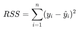
where :

yᵢ ​= observed value

ŷᵢ ​= predicted value from the model

• Interpretation: RSS represents the error or unexplained variability in the model. A smaller RSS indicates that the model's predictions are closer to the actual values, implying a better fit.

ESS (Explained Sum of Squares)

• ESS measures the variability in the data that is explained by the Model. It is the sum of the squared differences between the predicted values and the mean of the observed values.

• Formula:

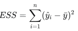
where :

ŷᵢ ​= predicted value

ȳ = mean of the observed values

• Interpretation: ESS represents the portion of the total variability that the model successfully explains. A higher ESS means the model captures more of the data’s structure, indicating a better explanatory power.

Relationship Between TSS, RSS and ESS

                                              TSS = ESS + RSS

This equation shows that the total variability in the dependent variable (TSS) is the sum of the explained variability by the model (ESS) and the unexplained variability or residual error (RSS).

Degree of Freedom (df)

In linear regression, the total degrees of freedom (df total) represent the total number of data points minus 1. It reflects the overall variability in the dataset that can be attributed to both the model and the residuals.

For a linear regression with n data points (observations), the total degrees of freedom is calculated as :

df total = n - 1

where :

• n = number of data points (observations) in the dataset

The total degrees of freedom in linear regression are divided into two components :

1. Degrees of Freedom for the Model (df model) :

   
   

This equals the number of independent variables in the model, typically denoted as K.

2. Degrees of Freedom for the Residual (df residual) :

This indicates the number of independent pieces of information available for estimating the variability in the residuals (errors) after fitting the regression model. It is calculated as the number of observations n minus the number of estimated parameters, which includes the intercept :

df residual = n - (K + 1)

The total degrees of freedom is the sum of model and residual degrees of freedom :

df total = df model + df residual

F-Statistic & Prob(F-Stat)

The F-test for overall significance is a statistical method used to determine whether a linear regression model is statistically meaningful—i.e., whether it provides a better fit to the data than simply using the mean of the dependent variable.

Steps to Conduct an F-Test for Overall Significance :

1. State the null and alternative hypothesis:

Null hypothesis (H₀): All regression coefficients (except the intercept) are equal to zero (β₁ = β₂ = … = βₖ = 0), meaning that none of the independent variables contribute significantly to the explanation of the dependent variable's variation.

Alternative hypothesis (H₁): At least one regression coefficient is not equal to zero, indicating that at least one independent variable contributes significantly to the explanation of the dependent variable's variation.

2. Fit the linear regression model to the data, estimating the regression coefficients (Intercept and slope).

3. Calculate the sum of squares (SS) :

• TSS (Total Sum of Squares): Total variation in the dependent variable.

• ESS (Explained Sum of Squares): Variation explained by the model.

• RSS (Residual Sum of Squares): Variation not explained by the model.

4. Compute the Mean Squares (MS) :

• Mean square Regression (MSR):

Where k = number of independent variables. It represents the average explained

variance per predictor.

• Mean square Error (MSE):

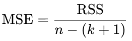
Where n = number of observations. This gives the average unexplained

        variance per degree of freedom.

5. Calculate the F-statistic :

                        F statistic = MSR/MSE

6. Determine the p-value associated with the F-statistic using the F-distribution or statistical software.

   
   

7. Compare the p-value to the significance level α :

   • If p-value < α, reject the null hypothesis. The model is statistically significant; at least one independent variable adds predictive power.

   • If p-value ≥ α, fail to reject the null hypothesis. This implies the model does not significantly outperform a model with no predictors.

Following these steps, you can perform an F-test for overall significance in a linear regression analysis and determine whether the regression model is statistically significant.

R-squared (R²)

R-squared (R²), also known as the coefficient of determination, is a metric used in regression analysis to evaluate the goodness-of-fit of a model. It quantifies the proportion of variance in the dependent variable (response variable) that is explained by the independent variable(s) (predictors) in the model.

R² values range between 0 and 1, with higher values indicating a better fit between the model and the observed data. In simple linear regression, R² is the square of the Pearson correlation coefficient (R) between the observed and predicted values. In multiple regression, R² is calculated from the ratio of the explained sum of squares (ESS) to the total sum of squares (TSS):

R² = ESS/TSS

Where:

• ESS (Explained Sum of Squares) is the sum of squared differences between the predicted values and the mean of the observed values. It represents the portion of variation in the response variable that is explained by the model.

• TSS (Total Sum of Squares) is the sum of squared differences between the observed values and their mean. It represents the total variation in the response variable.

Alternatively, R² can be expressed as :

Where:

• RSS (Residual Sum of Squares) is the portion of variation not explained by the model (the error).

Interpretation :

• An R² of 0 means the model explains none of the variation in the response variable.

• An R² of 1 means the model explains all of the variation.

Caution : A high R² does not always imply a good model, especially when irrelevant or excessive predictors are included. R² can be artificially inflated with more predictors, even if they are not statistically significant.

Adjusted R-squared (Adjusted R²)

Adjusted R-squared is a modified version of R-squared (R²) that adjusts for the number of predictor variables in a multiple regression model. It provides a more reliable measure of a model’s goodness-of-fit by accounting for model complexity.

In multiple regression, R² measures the proportion of variance in the response variable that is explained by the predictor variables. However, R² always increases or remains constant when new predictors are added — even if those predictors are irrelevant. This can lead to overfitting, where the model captures noise rather than meaningful relationships in the data.

Adjusted R² addresses this issue by incorporating both the number of predictors and the sample size, applying a penalty for adding unnecessary variables. Unlike R², Adjusted R² can decrease when irrelevant predictors are added, making it a better metric for comparing models with different numbers of variables.

Where:

• R² = R-squared of the model

• n = Number of observations in the dataset

• k = Number of predictor variables

Interpretation :

Adjusted R² helps you assess the true explanatory power of your model, free from the inflation that comes with merely adding more variables. It’s especially useful when performing model selection or comparing regression models with a different number of predictors.

Which One Should Be Used ?

The choice between using R-squared and adjusted R-squared depends on the context and the goals of your analysis. Here are some guidelines to help you decide which one to use:

1. Model Comparison :

   
   

   If you're comparing models with different numbers of predictor variables, it’s better to use adjusted R-squared. This is because adjusted R-squared takes into account the complexity of the model, penalizing models that include irrelevant predictor variables. R-squared, on the other hand, can be misleading in this context, as it tends to increase with the addition of more predictors, even if they don’t improve the model.

2. Model Interpretation :

   
   

   If you're interested in understanding the proportion of variance in the response variable that can be explained by the predictor variables, R-squared can be a useful metric. However, remember that R-squared does not indicate the significance or usefulness of individual predictors. Also, a high R-squared does not imply causation or confirm that the model will perform well on unseen data.

3. Model Selection and Overfitting :

   
   

   When avoiding overfitting and selecting predictor variables, it’s important to be cautious. In this context, adjusted R-squared can be a helpful metric, as it considers the number of predictors and penalizes unnecessary complexity. By using adjusted R-squared, you can avoid including irrelevant features that might lead to an overly complex model.

In summary :

• Adjusted R-squared is generally better for comparing models with different numbers of predictors and helps prevent overfitting.

• R-squared is useful for assessing overall explanatory power, but should be interpreted with caution when many predictors or multicollinearity are present.

T-statistic (T-test)

When creating a linear regression model, you may consider several different factors or independent variables. However, including too many variables can make the model unnecessarily complex. Therefore, it becomes important to select the most relevant predictors to make the model faster to train, easier to interpret, and less prone to multicollinearity. This is where hypothesis tests such as the t-test come into play, helping us calculate t-statistics for each coefficient.

The appropriateness of the linear relationship can be assessed by calculating the t-statistic for every regression coefficient. In regression models, the t-statistic helps determine whether a predictor is a meaningful contributor to the model.

The t-test checks whether the coefficients are significantly different from zero, indicating whether the corresponding variables have a statistically significant impact.

Steps to Perform a t-Test in Linear Regression (p-value approach):

1. State the null and alternative hypotheses :

For the slope coefficient (β₁) :

• Null hypothesis (H₀) : β₁ = 0 (no relationship between predictor X and response y)

• Alternative hypothesis (H₁) : β₁ ≠ 0 (a relationship exists)

For the intercept (β₀) :

• Null hypothesis (H₀) : β₀ = 0 (regression line passes through origin)

• Alternative hypothesis (H₁) : β₀ ≠ 0 (line does not pass through origin)

2. Estimate coefficients b₀ and b₁ :

   Use sample data to calculate the slope (b₁) and intercept (b₀) of the regression model.

   
   

3. Calculate the standard errors SE(b₀) and SE(b₁) :

   Compute the standard errors for the estimated coefficients using appropriate formulas.

4. Compute the t-statistics for slope and intercept :

   Use the formula:

5. Calculate the p-values :

   Using the calculated t-values and degrees of freedom (n − 2), find the corresponding p-values from the t-distribution (via table or statistical software).

   
   

6. Compare p-values to significance level (α) :Typically, α = 0.05 for a 95% confidence level.

   
   

7. Decision rule :

   If p-value ≤ α, reject the null hypothesis.

   If p-value > α, fail to reject the null hypothesis.

Confidence Intervals for Coefficients

Confidence intervals provide a range of plausible values within which the true population regression coefficients are likely to fall, based on sample data. Here's how to compute them for a simple linear regression model:

1. Estimate the slope and intercept coefficients (b₀, b₁) :

   Using the sample data, calculate the slope (b₁) and intercept (b₀) coefficients for the regression model.

2. Calculate the standard errors (SE(b₀) and SE(b₁)) :

   Compute the standard errors for the estimated slope and intercept using appropriate formulas derived from the residual sum of squares and the variability in the independent variable.

3. Determine the degrees of freedom (df) :

   In simple linear regression, degrees of freedom are calculated as:

df = n − 2

Where n is the number of observations, and 2 accounts for the estimated intercept

and slope.

4. Find the critical t-value (t) :

   Use a t-distribution table or a statistical calculator to find the critical t-value based on the desired confidence level (e.g., 95%) and the degrees of freedom.

5. Calculate the confidence intervals for the slope and intercept :

Use the following formulas:

• For the slope:

  CI(b₁) = b₁ ± t × SE(b₁)

• For the intercept:

  CI(b₀) = b₀ ± t × SE(b₀)

These confidence intervals define the range in which the true population regression coefficients (β₀ and β₁) are likely to lie, with a specified level of confidence (e.g., 95%). Narrower intervals indicate more precise estimates, while wider intervals reflect greater uncertainty due to data variability or small sample size.