Self-Attention in Transformers Explained from First Principles (With Intuition & Math)

How does self-attention work ?

Let us understand self-attention from first principles.

Consider two sentences: “money bank grows” and “river bank flows.” The word bank appears in both sentences, but its meaning is different—one refers to a financial institution, the other to a riverbank. If we use static word embeddings, the embedding for bank will be identical in both cases, which is undesirable because the context is different. Therefore, the meaning of a word must change based on its surrounding words.

Instead of representing bank as a single fixed vector, we represent it as a combination of other words present in its context. For example, in the first sentence, bank should be influenced more by money and grows, while in the second sentence it should be influenced by river and flows. Conceptually, we can think of bank as being formed from weighted contributions of neighboring words.

Using this idea, we can rewrite the sentences as follows.

First sentence:

• money = 0.7 money + 0.2 bank + 0.1 grows

• bank = 0.25 money + 0.7 bank + 0.05 grows

• grows = 0.1 money + 0.2 bank + 0.7 grows

Second sentence:

• river = 0.8 river + 0.15 bank + 0.05 flows

• bank = 0.2 river + 0.78 bank + 0.02 flows

• flows = 0.4 river + 0.01 bank + 0.59 flows

Here, every word is expressed as a weighted combination of other words in the same sentence. The key observation is that although bank appears in both sentences, the right-hand side is different, which means its representation now depends on context.

Since machines cannot operate directly on words, we move from words to word embeddings. Instead of writing these equations using words, we write them using embedding vectors.

First sentence:

• ε(money) = 0.7 ε(money) + 0.2 ε(bank) + 0.1 ε(grows)

• ε(bank) = 0.25 ε(money) + 0.7 ε(bank) + 0.05 ε(grows)

• ε(grows) = 0.1 ε(money) + 0.2 ε(bank) + 0.7 ε(grows)

Second sentence:

• ε(river) = 0.8 ε(river) + 0.15 ε(bank) + 0.05 ε(flows)

• ε(bank) = 0.2 ε(river) + 0.78 ε(bank) + 0.02 ε(flows)

• ε(flows) = 0.4 ε(river) + 0.01 ε(bank) + 0.59 ε(flows)

Each embedding ε(·) is an n-dimensional vector. A weighted sum of these vectors is also an n-dimensional vector, which makes this formulation mathematically valid. The coefficients (such as 0.7, 0.2, 0.1) indicate how strongly one word is related to another in a given context. For example, 0.7 represents high similarity between money and itself, while 0.2 captures partial similarity between money and bank in that sentence.

These similarity values are computed using dot products between embedding vectors. In practice, the dot product serves as a measure of similarity between two embeddings. Using these dot products, we can construct new contextual word embeddings.

To see this more clearly, consider the contextual embedding for bank in the first sentence:

ε(bank)⁽new⁾

= [ ε(bank) · ε(money)ᵀ ] ε(money)

• [ ε(bank) · ε(bank)ᵀ ] ε(bank)

• [ ε(bank) · ε(grows)ᵀ ] ε(grows)

Here, we take the dot product of the bank embedding with every word embedding in the sentence. These dot products produce scalar values (say s₂₁, s₂₂, s₂₃). Since raw dot products can have arbitrary magnitudes (for example, 36, −15, 32), we normalize them using the softmax function.

Applying softmax to s₂₁, s₂₂, and s₂₃ gives normalized weights w₂₁, w₂₂, and w₂₃, which sum to 1. We then compute the weighted sum:

ε(bank)⁽new⁾ = w₂₁ ε(money) + w₂₂ ε(bank) + w₂₃ ε(grows)

This new vector can be denoted as y_bank. It is the contextual embedding of bank, formed as a weighted combination of embeddings from the same sentence. The same procedure is applied to all other words.

This is the core first-principles intuition behind self-attention: each word attends to all other words in the sentence, computes similarity scores, normalizes them, and forms a new context-aware representation through a weighted sum.

Now let us review this method and highlight a few important points.

The first key point is that this operation is inherently parallel. While we conceptually describe computing the contextual embedding for the first word, then the second, then the third, there is no actual dependency that forces these computations to happen sequentially. All words in a sentence can be processed together. Using linear algebra, we can compute the contextual embeddings for all tokens in a single operation, even when the sentence is long.

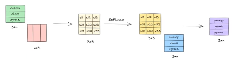
We usually write this process in matrix form. Suppose there are 3 words in the sentence and each word embedding is of dimension n. We stack the word embeddings into a matrix of shape 3 × n. We then multiply this with another matrix of shape n × 3, which gives a 3 × 3 matrix of dot products. After applying the softmax operation, we obtain a weight matrix W. Multiplying this weight matrix with the original word embedding matrix produces new combinations of embeddings. The important advantage here is that, regardless of how many words are present, we can generate all contextual embeddings in parallel in a single forward pass. This makes the method fast and computationally efficient.

However, parallelism also introduces a limitation. When all words are processed together, we lose explicit information about word order. From this operation alone, the model cannot directly infer which word comes first or last in the sentence. This is both an advantage (speed and scalability) and a disadvantage (loss of sequence information), and it is something that needs to be addressed separately.

The second important point is that no learnable parameters are involved in this formulation. In deep learning models, weights and biases enable learning from data. Here, we are only performing fixed linear algebra operations on embeddings. There are no parameters to update, which means there is effectively no learning. Given a word like hello, we can generate a contextual embedding based on surrounding words, but this process does not improve with more data.

The self-attention mechanism described so far is influenced only by the current input embeddings, not by the task or dataset. As a result, the contextual embeddings produced are general-purpose, not task-specific. For example, if we want to translate a sentence into Hindi, the same word can have different meanings depending on context and task. Using general contextual embeddings may not capture these task-dependent nuances, leading to suboptimal results.

This highlights a core limitation of this simple approach. While it successfully generates contextual embeddings and does so efficiently in parallel, the embeddings are not tailored to any specific task or dataset. General embeddings are not always sufficient across all tasks. To achieve better performance, especially in tasks like translation, classification, or question answering, embeddings need to be task-specific.

To address this, we introduce learnable parameters such as weights and biases. With learnable parameters, the self-attention mechanism can adapt based on data. When the model encounters new sentences, it can learn from examples and generate contextual embeddings that are better aligned with the task objective.

In summary, this first-principles self-attention approach works and efficiently produces contextual embeddings in parallel. Its major limitation is the absence of learning, which results in general, task-agnostic embeddings. By introducing learnable parameters, we enable the model to produce task-specific contextual embeddings and achieve better overall performance.

Now the goal is to introduce learnable parameters—such as weights and biases—so that the model can learn from data and generate task-specific embeddings rather than general ones. If we think about the earlier flow diagram logically, we need to identify where these learnable parameters can be inserted.

The basic self-attention computation consists of three steps: a dot product, followed by a softmax operation, and then another dot product. We cannot introduce learnable weights inside the softmax itself, so the only valid places to introduce parameters are in the dot-product operations.

At this point, an important observation emerges: each word embedding plays three different roles during the computation of its contextual embedding. Consider the word money while generating its contextual embedding. The same money embedding appears in three different forms at three different stages of the computation.

In the first step, the money embedding is used to measure similarity with all other words in the sentence. In the diagram, these are shown as the green boxes. Here, the embedding is effectively asking a question: How similar am I to the other words? In self-attention terminology, this role is called the query.

In the second step, the embeddings shown in pink represent the words that are being compared against the query. These embeddings determine how relevant each word is to the current query word. In this role, the embeddings act as keys—the query is matched against these keys to compute similarity scores.

In the final step, once the similarity scores are normalized into weights, we compute a weighted sum of embeddings (shown in blue). These embeddings provide the actual information that gets aggregated. In self-attention terminology, they are called values.

So, to compute a contextual embedding, the process is intuitive: the query asks for similarity, the keys provide matching scores, and the values provide the content that gets combined. The same word embedding is reused in three different ways—as a query, as a key, and as a value. This applies not only to money but also to bank, grows, and every other word in the sentence.

The naming of query, key, and value comes directly from common computer science terminology. For example, consider a Python dictionary {a:1, b:3, c:4}. Here, a, b, and c are keys, and 1, 3, and 4 are values. If the dictionary is d, then d[a] is a query that asks for the value associated with key a.

Self-attention follows the same idea. To compute a contextual embedding, a word embedding issues a query to other embeddings. Those embeddings act as keys, and the responses they provide are the values. For every word in the sentence, its embedding participates in all three roles—query, key, and value—during the computation.

This clear separation of roles allows us to introduce learnable weight matrices for queries, keys, and values. With these learnable parameters, the model can adapt based on data and learn task-specific contextual embeddings, rather than relying on fixed, general-purpose representations.

Query, Key, and Value Vectors

In the earlier formulation, a key limitation is that a single embedding vector is being used to play the roles of query, key, and value. Ideally, these should be three different vectors derived from the same embedding. This separation of concerns allows each vector to specialize in its role. Expecting one vector to perform all three functions simultaneously is inefficient; transforming it into three different representations allows each role to be performed more effectively. Hence, from a single word embedding (for example, bank), we should derive three vectors:

q_bank (query), k_bank (key), and v_bank (value).

To build intuition, consider the following analogy.

Suppose there is a person who is an author and has written many books. Recently, he writes his autobiography describing his experiences and personality. At the age of 35, his parents want him to get married, so he joins a matrimonial website. On such a platform, three distinct activities take place.

First, a profile is created. This profile is designed so that others can discover him based on their preferences. Second, there is search, where users look for potential matches by querying the system based on specific criteria. Third, there is matching and interaction, where people communicate and decide whether the relationship should progress.

In this analogy, the autobiography corresponds to the original word embedding. The act of searching—where similarities are computed—is analogous to the query in the attention mechanism. The profile represents the key, which stores structured information used for matching. Finally, the actual interaction or match corresponds to the value, which provides the meaningful content once a match is made.

In the initial setup, using the same embedding for query, key, and value is equivalent to uploading the entire autobiography everywhere. If the person refuses to create a proper profile, nobody can discover him. If he pastes his entire autobiography into the search bar, the system cannot understand what he is actually looking for. And if, after matching, he asks others to read his entire autobiography instead of communicating directly, it may lead to misunderstandings or poor outcomes. Clearly, using the same information in all three places is not logical.

Similarly, in self-attention, using a single embedding vector for query, key, and value is not ideal. Each role requires different information. A good profile highlights only relevant traits. A good search query reflects personal preferences. Effective communication after matching focuses on the most meaningful aspects. All of these improve over time by learning from experience.

In the same way, from a word embedding we should extract three different pieces of information: one for querying, one for matching (keys), and one for aggregation (values). These are learned from data. Initially, the profile or query may be poorly designed, but over time—based on feedback and outcomes—it improves. Preferences change, queries get refined, and matching behavior becomes more effective.

This is exactly what learnable query, key, and value projections enable in attention models. The vectors Q, K, and V are learned from data so that the model improves its similarity matching, information retrieval, and contextual representation over time. Each embedding vector thus plays three roles, but through three different learned transformations, allowing the attention mechanism to adapt and perform effectively based on data.

How to build vectors from an embedding vector

Consider the sentence “money bank grows.” For self-attention, each word embedding must be transformed into three separate vectors: a query vector, a key vector, and a value vector. These three vectors allow the model to ask questions (query), compare relevance (key), and aggregate information (value).

If we want to compute the contextual embedding for the word money, we first create three vectors from its original embedding: q_money, k_money, and v_money. Since the sentence has three words, each word produces three vectors, giving a total of 3 × 3 = 9 vectors for the sentence.

Earlier, we directly used the word embeddings to compute attention. Now, instead of using the raw embeddings, we use their query, key, and value components. To compute the contextual embedding for money, we send the query vector of money and compare it with the key vectors of all words in the sentence. After computing similarities and applying softmax, we use the resulting weights to combine the value vectors and obtain the final contextual embedding for money.

The same procedure is repeated for the other words in the sentence. In this way, each word gets its own contextual embedding, influenced by all other words.

At this stage, we successfully obtain contextual embeddings using query, key, and value vectors.

The remaining question is important: given a single embedding vector, how do we generate these three different vectors? In other words, what mathematical operation allows one embedding to be transformed into separate query, key, and value representations?

How these vectors are computed

Now let us see how these vectors are actually obtained.

We start with a single embedding vector and need to generate three different vectors from it: a query vector, a key vector, and a value vector. This is achieved through linear transformations. A linear transformation changes both the magnitude and direction of a vector by multiplying it with a matrix, which makes it a suitable and flexible operation for this purpose.

Suppose we have an embedding vector e₍bank₎. We multiply this vector with three different matrices to obtain three new vectors:

Query vector:

q₍bank₎ = W_q · e₍bank₎

Key vector:

k₍bank₎ = W_k · e₍bank₎

Value vector:

v₍bank₎ = W_v · e₍bank₎

Here, W_q, W_k, and W_v are learnable weight matrices. Each matrix transforms the same embedding vector in a different way, producing vectors that are specialized for querying, matching, and information aggregation.

A natural question is: where do the numbers inside these matrices come from?

These values are learned from data. During training, the matrices are typically initialized with random values. We pass sentences through the model, generate predictions (for example, translations or next-word predictions), and compute errors. These errors are then propagated backward using backpropagation, and the weights in W_q, W_k, and W_v are updated.

This process is repeated many times, and gradually the matrices learn meaningful transformations. Once training converges, these matrices contain values that produce effective query, key, and value vectors for a given task.

This process is applied to every word in the sentence, but an important detail is that the same weight matrices W_q, W_k, and W_v are reused for all words. The matrices used for money are exactly the same ones used for bank, grows, and every other token. This shared transformation is what defines the self-attention mechanism.

In practice, we stack all word embeddings of a sentence into a single matrix and multiply it three times with W_q, W_k, and W_v. This produces the Q, K, and V matrices in one shot. We then compute similarity scores by multiplying Q with the transpose of K (Kᵀ), apply the softmax function to normalize these scores, and finally multiply the result with V.

The output is the final contextual embedding for each word.

All of these operations are matrix multiplications, which means they can be executed efficiently and in parallel, typically using GPUs. This parallelism is one of the key reasons self-attention is both powerful and scalable, while also producing task-specific contextual embeddings learned directly from data.