Support Vector Machine (SVM) – Part 6

Dual Formulation of SVM

The dual optimization problem for a hard-margin Support Vector Machine is :

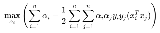
Important Notes :

• αᵢ = 0 for non-support vectors

• αᵢ > 0 for support vectors

This means only the support vectors contribute to the model parameters (e.g., w and the decision function).

Understanding the Dual Form with an Example

Suppose we are given a dataset with corresponding margins, model lines, and identified support vectors.

For every data point xᵢ , there exists a corresponding Lagrange multiplier αᵢ . However, only the support vectors have αᵢ > 0 ; all non-support vectors have αᵢ = 0. This is crucial to the dual formulation : it ensures that only support vectors influence the decision boundary.

Dual Objective Breakdown

If we assume there are five support vectors, then in the dual objective function :

Only the five non-zero αᵢ's contribute. So the first term simplifies to :

The second term involves all pairwise dot products of support vectors only, as all other αᵢαⱼ terms will be zero.

Sample Data Format

Assume the feature vectors and labels are structured as :

We use only these five support vectors in our dual formulation. This drastically reduces the complexity of computation.

Grid-Based Computation View

We can think of computing the second term in a 5×5 grid , where each cell corresponds to a pairwise interaction between support vectors :

There are 5×5 = 25 such terms in the sum for the second term of the dual.

Summary

• In the dual form, only support vectors contribute to the optimization problem.

• The dot products xᵢᵀxⱼ are calculated only for support vectors.

• This makes the computation faster and more efficient than in the primal, which considers all data points.

• This is why it's called Support Vector Machine: only a subset (support vectors) determines the model.

The Similarity Perspective in SVM Dual Form

The cosine similarity between two vectors A and B is defined as :

If both vectors are normalized (i.e., ∥A∥=∥B∥=1), this simplifies to :

Cosine similarity = A⋅B

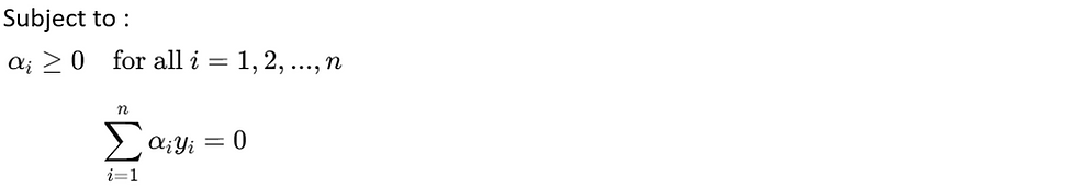
In the dual form of the Support Vector Machine (SVM) optimization problem, we have :

Here, the term xᵢ · xⱼ represents the dot product of two input vectors.

If we assume that each xᵢ and xⱼ is normalized (i.e., unit vectors), then xᵢ · xⱼ becomes the cosine similarity between them. This allows us to reinterpret the objective function geometrically :

• We are maximizing a combination of similarity terms between data points.

• These similarity terms are weighted by αᵢαⱼyᵢyⱼ .

• The sign and magnitude of these weights encode how the similarity contributes to maximizing the margin.

Geometric Intuition

Thus, in the dual form, we are effectively computing and optimizing over pairwise similarities (dot products) between vectors, especially those that become support vectors. The learning algorithm seeks to maximize similarity between similarly labeled vectors and minimize it otherwise—this leads to a maximum margin classifier.

Connection to the Kernel Trick

Now, extending this idea, the dot product xᵢ · xⱼ is essentially a measure of linear similarity. But what if we want to measure similarity in a non-linear space ?

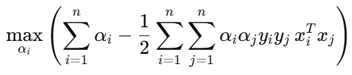
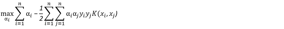
We generalize this by introducing a kernel function K(xᵢ , xⱼ), where :

This kernel function replaces the dot product with other forms of similarity, such as polynomial, RBF (Gaussian), or sigmoid kernels. This is the core of the kernel trick : we compute similarity in a higher-dimensional (possibly infinite-dimensional) space without explicitly computing the mapping ϕ .

KERNEL SVM

Dual SVM Formulation

What Is a Kernel ?

In Support Vector Machines (SVMs), K(xᵢ , xⱼ) is called a kernel function.

• It measures similarity between two input vectors xᵢ ​and xⱼ .

• However, it measures similarity in a higher-dimensional space — without actually computing that space.

This is different from the usual dot product, which finds similarity in the original input space.

Linear SVM vs Kernel SVM

• Linear SVM

  • Uses the dot product : xᵢ . xⱼ

  • Assumes that the data is linearly separable in the original input space.

  • No explicit kernel function is used.

  • Faster and works well when a straight-line (or hyperplane) separation is sufficient.

• Kernel SVM

  • Replaces the dot product with a kernel function: K(xᵢ , xⱼ)

  • Allows SVM to operate in an implicit higher-dimensional space.

  • Can separate non-linearly separable data using linear separators in the transformed space.

  • Examples: Polynomial kernel, RBF kernel, Sigmoid kernel, etc.

Summary :

When we replace the dot product with a kernel function, we call it a Kernel SVM.

If no kernel is used (i.e., we use the plain dot product), it is simply called a Linear SVM.

 Polynomial Kernel

When data is not linearly separable in its current form, a linear decision boundary (like a straight line) cannot classify the data effectively. For example :

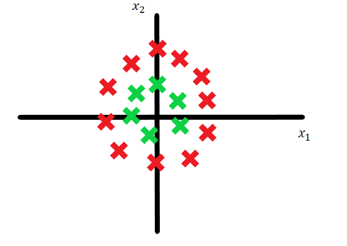
Why Use Polynomial Kernel ?

To handle such problems, we can transform our data into a higher-dimensional space. Consider this transformation :

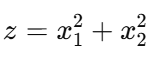
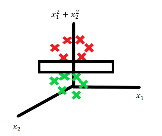
This maps each point from 2D into a 3D space (x₁, x₂, z), where :

• Green points have a lower value of z, because they are near the origin.

• Red points, farther from the origin, have a higher value of z.

In this higher-dimensional space, a hyperplane can now separate the data.

Mathematics Behind Polynomial Kernel

To avoid computing the transformation explicitly, we use the kernel trick.

The polynomial kernel is defined as :

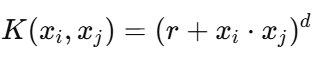
Where :

• xᵢ and xⱼ are two feature vectors,

• r is a constant (commonly set to 1),

• d is the degree of the polynomial (chosen based on the problem).

Let’s assume :

• r = 1

• d = 2

Worked Example

Suppose :

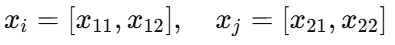
Then the kernel becomes :

Now expand this :

This expansion shows that we’re implicitly computing terms like squares and cross-products—just as if we had transformed the original data into a higher-dimensional space explicitly.

Conclusion

If we used a linear SVM, we would only compute the dot product xᵢ · xⱼ . But by using the polynomial kernel, we introduce polynomial terms without explicitly transforming the data.

This allows the SVM to :

• Work in higher-dimensional feature spaces

• Discover non-linear decision boundaries

• Find a solution even for complex datasets

The Trick — Understanding the Kernel Trick in SVM

Let’s discuss the kernel trick—a core idea in SVMs that allows us to build non-linear decision boundaries efficiently.

What is the "Trick" ?

The trick is that :

We do not explicitly transform the data to a higher-dimensional space.

Instead, we compute the result of operations as if the transformation had happened, while staying in the original low-dimensional space.

This is useful because calculating and storing high-dimensional vectors is expensive, but using a kernel function helps simulate those operations without ever constructing the high-dimensional vectors.

Why is this Important ?

SVMs use dot products of data points extensively in their calculations to find the best separation boundary. When we "lift" the data into a higher dimension using a feature map (let's call it ϕ), the SVM needs to calculate ϕ(point A)⋅ϕ(point B).

Explicitly calculating ϕ(point A), then ϕ(point B), and then their dot product can be computationally expensive and require a lot of memory, especially if the higher dimension is very, very large (which it can be!).

The Two Ways (and why the second is better) :

1. The Hard Way (Without the Trick) :

• Take your original low-dimensional points (x₁ , x₂​).

• Explicitly calculate their high-dimensional mapped versions (ϕ(x₁) , ϕ(x₂)). If your original data was 10D and you use a degree-2 polynomial mapping, these vectors could become 66D! If you had a million data points, you'd need to store a million 66D vectors – that's a lot of memory!

• Calculate the dot product between these large high-dimensional vectors (ϕ(x₁) . ϕ(x₂)). This takes time proportional to the high dimension.

2. The Smart Way (With the Kernel Trick) :

• Take your original low-dimensional points (x₁ , x₂).

• Apply a kernel function, which is a shortcut formula, to these original points. For this example, the kernel function K(x₁ , x₂) = (1 + x₁ · x₂)².

• Calculate K(x₁ , x₂) using only the low-dimensional coordinates. This calculation is much faster and uses far less memory because you never create or store the high-dimensional vectors.

The Key Takeaway :

The kernel trick is a computational shortcut. It allows SVMs to find complex, non-linear decision boundaries by implicitly working in a high-dimensional feature space, but it does so by calculating the necessary dot products using a kernel function that operates directly on the original, lower-dimensional data. We get the power of high dimensions without the computational and memory cost of explicitly going there. That's why it's called a "trick"!

Understanding Polynomial Kernels in SVMs

When dealing with data that is not linearly separable in its original space, Support Vector Machines (SVMs) can use a technique called the "kernel trick." This involves implicitly mapping the data into a higher-dimensional feature space where it is linearly separable. The polynomial kernel is one way to achieve this mapping.

The core idea is that a linear boundary in this higher-dimensional space can correspond to a non-linear boundary in the original space.

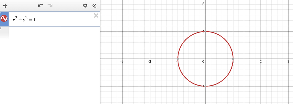
1. The Challenge of Non-Linear Data and the Mapping Concept

Consider data that cannot be separated by a straight line in its original 2D space, such as data arranged in concentric circles.

The strategy is to map these data points into a higher-dimensional space where they become linearly separable.

This mapping is done by a function ϕ that transforms the original feature vector x = [x₁, x₂, ..., xₙ] into a higher-dimensional feature vector ϕ(x).

2. The Polynomial Kernel and Implicit Mapping

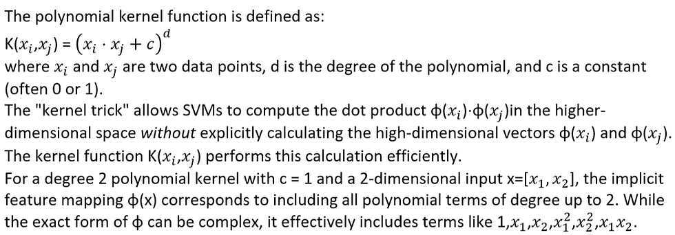
3. The Kernel Expansion Explains the Terms

4. Why Include All Terms ? The Benefit of Diverse Features

The Role of Additional Terms

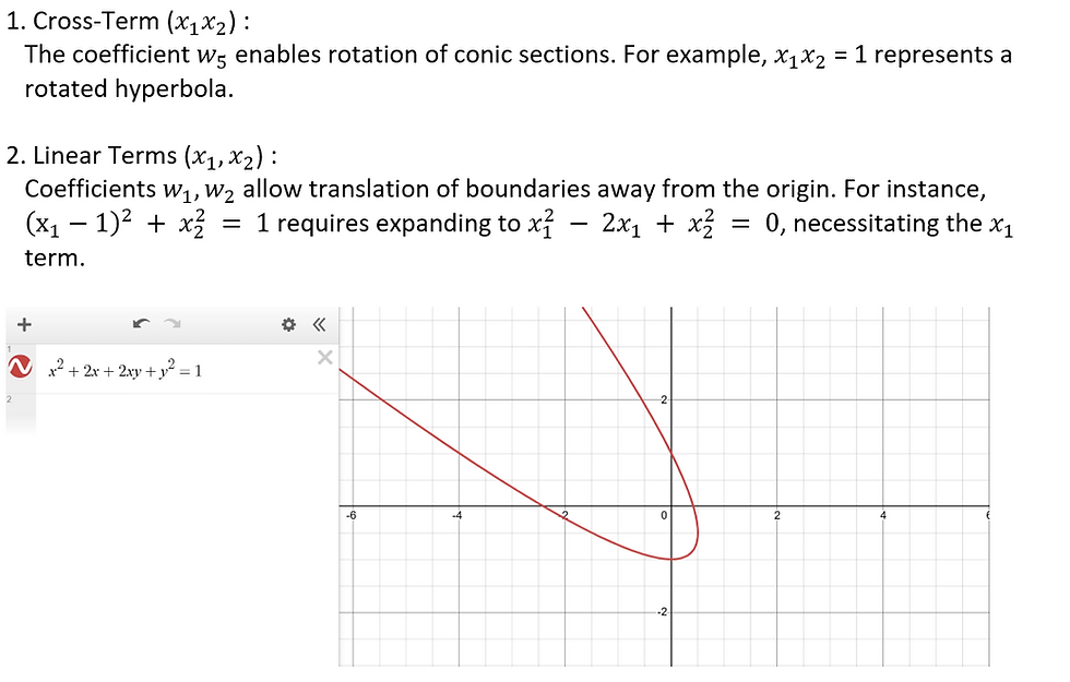
Why Full Polynomials Matter

Including all terms up to degree d allows the SVM to represent arbitrary degree-d polynomial boundaries. For d = 2, this means any conic section—rotated, translated, scaled, or degenerate—can be learned, maximizing the model's flexibility.

Conclusion

By including all terms in the polynomial kernel expansion (which is implicitly done by using the kernel function), we empower the SVM to find a linear boundary in the rich, higher-dimensional space that translates to a flexible non-linear boundary in the original space. This flexibility, allowing for shapes like general conic sections, is crucial for accurately separating data that requires such complex boundaries.

RBF KERNEL

The full form of RBF is Radial Basis Function. It is mathematically similar to the Gaussian (Normal) distribution. The RBF kernel is extremely popular and is often the default kernel used in Support Vector Machines (SVMs). It is highly effective and works well “out of the box.”

Benefits of the RBF Kernel :

• Non-linear Transformations : The RBF kernel enables the use of non-linear transformations, which can map the original feature space to a higher-dimensional space where the data becomes linearly separable. This is particularly useful for problems where the decision boundary is not linear.

• Local Decisions : Unlike some other kernels, the RBF kernel makes "local" decisions. That is, the effect of each data point is limited to a certain region around that point. This can make the model more robust to outliers and create complex decision boundaries.

• Flexibility : The RBF kernel has a parameter (related to the standard deviation of the Gaussian distribution) that determines the complexity of the decision boundary. By tuning this parameter, we can adjust the trade-off between bias and variance, allowing for a flexible range of decision boundaries.

• Universal Approximation Property : The RBF kernel has a property known as the universal approximation property, meaning it can approximate any continuous function to a certain degree of accuracy given enough data points. This makes it highly versatile and capable of modeling a wide variety of relationships in data.

• General-Purpose : The RBF kernel does not make strong assumptions about the data and can therefore be a good choice in many different situations, making it a versatile, general-purpose kernel.

RBF Kernel — Mathematical Derivation & Interpretation

To compute the RBF (Radial Basis Function) kernel, we need to provide two vectors (e.g., support vectors) as inputs. The kernel function computes a similarity measure based on the Euclidean distance between these two vectors.

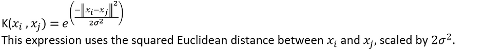
Formula of the RBF Kernel

The standard formula is :

Rewriting in Terms of Gamma

We define :

This allows us to simplify the kernel expression to :

In scikit-learn, γ is a hyperparameter that controls the smoothness of the decision boundary.

Interpretation as a Similarity Function

Let’s understand the kernel as a similarity function.

• The term ||xᵢ − xⱼ|| is the Euclidean distance between the two points.

• So, we can rephrase the kernel formula as : 

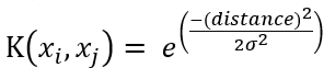
This shows how the kernel value changes based on the distance between vectors.

Relationship Between Distance and Kernel Value

• As distance increases, the exponent becomes more negative ⇒ kernel value decreases.

• As distance decreases, the exponent becomes less negative ⇒ kernel value increases.

Thus, we observe :

This means :

• High similarity (K ≈ 1) when xᵢ ≈ xⱼ (small distance).

• Low similarity (K ≈ 0) when xᵢ and xⱼ are far apart.

Hence, RBF kernel acts as a similarity function that assigns higher weights to closer points.

Local Decision Boundary

To understand the local behavior of the RBF kernel, we analyze the function :

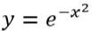
This graph helps visualize how similarity (kernel value) decays with distance.

Understanding the Graph

• X-axis: Represents the distance between two points.

• Y-axis: Represents the similarity or kernel value.

We observe how similarity changes as the distance between two vectors increases.

Key Observations

• When distance = 0, we get :

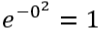
This is the maximum similarity — the points are identical.

• When distance = 0.5, similarity decreases but remains significantly high.

• When distance = 1, similarity further decreases.

• At distance ≈ 2, the similarity is very close to zero.

• For distance > 2, similarity is effectively zero, meaning the two points are treated as completely different.

Intuition Behind Locality

• The RBF kernel is a local similarity function.

• It gives high similarity only to nearby points (within a certain range).

• For |distance| > 2, the kernel value is almost zero ⇒ no meaningful influence.

Summary