Support Vector Machine (SVM) – Part 5

SVM in N Dimensions

So far, we have studied Support Vector Machines (SVMs) in the context of 2D, where we draw a line defined by the equation :

AX + BY + C = 0 

Now, we will extend the concept of SVM to n-dimensional space.

In this scenario, we have n input features and one output label.

In higher dimensions, instead of a line, the decision boundary becomes a hyperplane.

The general form of a hyperplane in n dimensions is :

Or, more compactly :

To find the optimal separating hyperplane, we need to determine the values of w and b that maximize the margin while allowing some misclassifications (soft margin).

Soft Margin SVM in 2D

The soft-margin optimization problem for 2D data is :

Subject to :

Generalizing to N Dimensions

We now extend this formulation to n dimensions :

Subject to :

For mathematical convenience, we replace ∥w∥ (norm) with ||w||². This simplification does not affect the optimization outcome but makes derivative calculations more tractable.

Subject to :

This is the soft-margin SVM optimization problem in n dimensions— the foundational formula we'll be working with.

Constraint Optimization Problems with Inequality

In the previous section, we learned how to solve constraint optimization problems involving equality constraints using methods such as Lagrange multipliers.

However, this is not sufficient for our purposes — particularly in Support Vector Machines (SVMs)— because SVMs involve inequality constraints. So, in this section, we will focus on solving constraint optimization problems that include inequality conditions.

Example Problem :

We consider a simple optimization problem :

This means we want to minimize f(x) = x^2under the constraint that :

This introduces an inequality constraint into the optimization problem.

Introducing the Karush-Kuhn-Tucker (KKT) Conditions

To handle inequality constraints systematically, we use the Karush-Kuhn-Tucker (KKT) conditions, which generalize Lagrange multipliers to optimization problems involving inequalities.

They generalize the method of Lagrange multipliers to handle inequality constraints. In the context of support vector machines (SVMs) and many other optimization problems, the KKT conditions play a key role in deriving the dual problem from the primal problem. The KKT conditions are :

1. Stationarity : The derivative of the Lagrangian with respect to the primal variables, the dual variables associated with inequality constraints, and the dual variables associated with equality constraints are all zero.  

2. Primal feasibility : All the primal constraints are satisfied.

3. Dual feasibility : All the dual variables associated with inequality constraints are nonnegative.

4. Complementary slackness : The product of each dual variable and its associated inequality constraint is zero. This means that at the optimal solution, for each constraint, either the constraint is active (equality holds) and the dual variable can be nonzero, or the constraint is inactive (strict inequality holds) and the dual variable is zero.

This prepares us to handle inequality-constrained problems like those found in SVM formulations. Let me know when you're ready to proceed to the next part or need elaboration on the example using KKT conditions step-by-step.

KKT Conditions and Their Use in SVM Dual Problem

The Karush-Kuhn-Tucker (KKT) conditions are used when solving optimization problems that involve inequality constraints. They are an extension of the Lagrange multipliers method and introduce specific conditions that must be satisfied for a solution to be optimal.

In the context of Support Vector Machines (SVM), KKT conditions play a critical role in solving the dual problem.

Understanding KKT with an Example

Let’s consider a simple constrained optimization problem :

This is our primal problem.

Note : The primal problem refers to the original constrained optimization problem.

Step 1 : Formulate the Lagrangian

To handle the inequality constraint, we form the Lagrangian function :

Here:

• λ ≥ 0 is the Lagrange multiplier for the constraint x−1 ≤ 0.

• This Lagrangian converts our constrained problem into an unconstrained one using penalty terms.

KKT Conditions

For inequality constraints, the KKT conditions consist of four key conditions :

1. Stationarity

   Take the partial derivative of the Lagrangian with respect to the primal variable x and set it to zero :

2. Primal Feasibility

   The original constraint must be satisfied :

   x−1 ≤ 0

3. Dual Feasibility

   The Lagrange multiplier must be non-negative :

   λ ≥ 0

4. Complementary Slackness

   The product of the constraint function and its corresponding multiplier must be zero :

                        λ(x−1) = 0

   This condition ensures that either the constraint is active (x=1) or the multiplier is zero (λ = 0).

   
   

To solve an optimization problem with inequality constraints :

• Start with the primal formulation.

• Construct the Lagrangian.

• Derive the stationarity condition by taking derivatives w.r.t  primal variables.

• Apply the KKT conditions :

  • Stationarity

  • Primal feasibility

  • Dual feasibility

  • Complementary slackness

Only the values of x and λ that satisfy all four KKT conditions are considered valid optimal solutions.

KKT Conditions — Example

Let’s solve the following constrained optimization problem using KKT conditions :

Step 1 : Construct the Lagrangian

We introduce a Lagrange multiplier λ ≥ 0 for the inequality constraint and write the Lagrangian :

Step 2 : Apply KKT Conditions

There are four conditions to check :

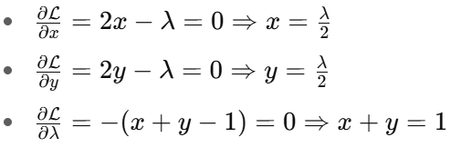
1. Stationarity :

Take partial derivatives of the Lagrangian and set them to zero :

2. Primal Feasibility :

   The constraint must be satisfied :

                                            x+y−1 ≤ 0

3. Dual Feasibility :

   The Lagrange multiplier must be non-negative :

                                            λ ≥ 0

4. Complementary Slackness :

                                         λ(x+y−1) = 0

   Step 3 : Solve the System

   From stationarity :

From primal constraint (now treated as equality due to complementary slackness) :

Substitute λ = 1 back :

Step 4 : Verify All KKT Conditions

• Primal Feasibility : x+y−1 = 0 ≤ 0

• Dual Feasibility : λ = 1 ≥ 0

• Complementary Slackness : λ(x+y−1) = 1(0) = 0

Conclusion

The solution :

x = 0.5 , y = 0.5 , λ = 1

satisfies all four KKT conditions. Hence, it is the optimal solution to the constrained optimization problem.

CONCEPT OF DUALITY

The duality principle is fundamental in optimization theory. It provides a powerful tool for solving difficult or complex optimization problems by transforming them into simpler or easier-to-solve problems. The solution to the dual problem provides a lower bound on the solution of the primal problem. If strong duality holds (i.e., the optimal values of the primal and dual problems are equal), then solving the dual problem can directly give the solution to the primal problem.

Solving the primal optimization problem directly in Support Vector Machines (SVMs) can often be difficult due to constraints and the form of the objective function. This is where the concept of duality becomes useful. By converting the primal problem into its dual form, we often obtain a simpler problem that is easier to solve, especially when the number of constraints is smaller than the number of variables.

There is a strong relationship between the primal and dual problems in SVM. In fact, solving the dual problem not only simplifies the computation but also provides the optimal solution to the original primal problem. This dual formulation also allows us to handle kernels more naturally, which is essential for non-linear SVMs.

Therefore, in the context of SVMs, we make use of duality to :

• Efficiently compute the solution for the optimization problem,

• Find the optimal weights w and bias b, and

• Leverage kernel methods for non-linear classification.

What’s Next ?

Now, let’s learn how to derive the dual problem from the primal formulation step by step.

SVM Dual Problem

Primal Form of Hard Margin SVM

In this formulation :

• w is the weight vector,

• b is the bias term,

• xᵢ are the training samples,

• yᵢ ∈ {−1,1} are the corresponding class labels.

The objective is to maximize the margin while ensuring that all data points are correctly classified with a margin of at least 1.

Dual Form of Hard Margin SVM

The dual form is derived from the primal using the method of Lagrange multipliers. It shifts the optimization from the w and b space to the space of Lagrange multipliers αᵢ , which are known as dual variables.

In the dual :

• The variables w and b disappear from the objective function.

• The optimization is entirely in terms of αᵢ .

• The data appears in the form of dot products xᵢ . xⱼ , which is important when introducing kernels.

Primal Form of Soft Margin SVM

Soft margin SVM allows some misclassification using slack variables ξᵢ . Its primal form is :

Here, the optimization balances maximizing the margin and minimizing the penalty for misclassification. The parameter C controls this trade-off.

Dual Form of Soft Margin SVM

The dual form of the soft margin SVM is :

Compared to the hard margin case :

• The key difference is in the bounds of αᵢ :

  • For hard margin: αᵢ ≥ 0

  • For soft margin: 0 ≤ αᵢ ≤ C

• The overall structure of the dual remains almost the same.

Summary Comparison

As observed, the dual forms of both hard and soft margin SVMs are nearly identical, with the only major difference being the constraint on αᵢ :

This demonstrates the mathematical elegance of duality—despite different primal forms, the dual formulations are structurally similar.

Next, we will derive the dual form step-by-step from the primal formulation.

Dual Problem Derivation

We are going to derive the dual formulation of the Support Vector Machine (SVM). We will start with the primal form of the hard-margin SVM.

The primal optimization problem is :

Subject to the constraints :

Since there is one constraint for each training example, we have a total of n constraints.

To form the Lagrangian, we introduce Lagrange multipliers αᵢ ≥ 0, one for each constraint. Therefore, the Lagrangian becomes a function of w, b, and the vector of Lagrange multipliers α = (α₁, α₂, ..., αₙ) .

The Lagrangian is defined as :

Conditions for Optimality

To find the saddle point of the Lagrangian, we take partial derivatives with respect to the primal variables w and b, and set them to zero :

1. Derivative with respect to w :

2. Derivative with respect to b :

Substituting Back into the Lagrangian

We now substitute equations (1) and (2) back into the Lagrangian :

The Dual Optimization Problem

The dual problem is to maximize the Lagrangian with respect to α, subject to the constraints ​αᵢ ≥ 0 (from the definition of Lagrange multipliers for inequality constraints) and the constraint derived from the partial derivative with respect to b.

This is the dual form of the SVM optimization problem, expressed entirely in terms of the Lagrange multipliers αᵢ ​and the dot products of the input data points .

OBSERVATIONS

Why Use the Dual Form ?

Let’s discuss the benefits of transforming the problem from primal to dual form in Support Vector Machines (SVMs).

Two Main Benefits of the Dual Form :

1. Simplified Optimization :

   The dual formulation is often easier to solve numerically, especially when the number of features is large compared to the number of training samples.

2. Kernel-Friendly Formulation :

   The dual involves dot products xᵢ · xⱼ , making it naturally compatible with the kernel trick. This allows SVMs to work efficiently in high-dimensional or even infinite-dimensional spaces without explicitly transforming the data.

Why is the Dual Easier to Solve ?

We previously derived that :

This means the weight vector w, which is required for classification, is constructed directly from the training data using only the support vectors(those with αᵢ > 0).

So instead of solving for w in the high-dimensional space directly, we optimize over αᵢ ​—a scalar for each training example—which simplifies the problem.

Recap of w in Terms of Support Vectors :

Only support vectors contribute to w, because for non-support vectors , αᵢ = 0 .

•  Alpha αᵢ > 0 only for support vectors – this simplifies computation and the final classifier.

•  The objective depends only on dot products xᵢ · xⱼ – which enables kernelization without explicit feature transformation.

Support Vectors in Dual Formulation

As we studied earlier, in SVM the decision boundary (also known as the model line) is defined by :

We’ve seen that the margin and decision boundary are determined only by the support vectors — the critical points that lie closest to the margin.

However, in the dual formulation, the expression for the optimal weight vector w is :

At first glance, this suggests that all training points contribute to w, since the summation runs over all n points. But this appears to contradict what we learned in the primal form, where only support vectors influence the decision boundary.

So, what’s going on ? Is there a contradiction ?

No Contradiction — Here's Why :

The key lies in the Lagrange multipliers αᵢ :

• For support vectors , αᵢ > 0

• For non-support vectors , αᵢ = 0

This is because the dual problem includes the constraint :

In the optimization process, only those points that lie exactly on the margin — the support vectors — will receive non-zero αᵢ . All other points contribute αᵢ = 0 , meaning they do not influence w.

illustrative Example :

Suppose :

• α₁y₁x₁ is a green support vector

• α₃y₃x₃ is a red support vector

• All other points (non-support vectors) have αᵢ = 0

Then :

This shows clearly that only support vectors contribute to the weight vector w.

Why the Dual is Efficient :

In the dual form of SVM, the optimization involves computing :

While this double summation seems to include all pairs of points, in practice, most αᵢ and αⱼ are zero, because only a small number of support vectors remain with non-zero multipliers.

So, during computation:

• Terms involving non-support vectors cancel out (since α = 0)

• Only terms involving support vectors remain

This makes the dual form computationally efficient because it focuses only on the most critical points — the support vectors — which are typically a small subset of the data.

Conclusion

So, there is no contradiction :

• In the primal form, it is conceptually clear that only support vectors determine the decision boundary.

• In the dual form, even though the summation goes over all data points, the math naturally eliminates non-support vectors by assigning them zero weight (α = 0).

That’s exactly why the algorithm is called a Support Vector Machine — because the model entirely depends on the support vectors.