Transformer Encoder Architecture Explained Step by Step (With Intuition)

SIMPLIFIED REPRESENTATION

This diagram represents the architecture of the Transformer. It has an encoder–decoder architecture, where the model is divided into two main parts: the encoder and the decoder. To make things easier to understand, we can first look at a simplified representation of this structure.

Now let’s add some complexity. In the diagram, the encoder and decoder blocks are marked with N×. This means that instead of having a single encoder block and a single decoder block, we have multiple stacked encoder and decoder blocks. In the original Attention Is All You Need paper, the Transformer uses six encoder blocks and six decoder blocks.

Even with this stacking, the structure still consists of an encoder part and a decoder part. We have six encoders and six decoders, and all of these blocks are identical in terms of their internal architecture. This means that if we understand how one encoder block works, we essentially understand how all encoder blocks work. So, we will now focus on understanding a single encoder block. Each encoder block mainly contains two key components: a self-attention block and a feed-forward neural network. Let’s understand what happens inside this block.

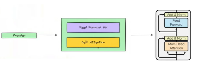
Now we can look at the actual representation of the encoder block. Inside the encoder block, we have a self-attention block followed by a feed-forward neural network, but there are additional connections as well. Specifically, we have Add & Norm operations along with residual connections.

If we zoom out and observe the encoder as a whole, the flow becomes clear. The input is sent to the first encoder block, its output is passed to the second encoder block, the output of the second goes to the third as input, and this process continues sequentially. After the sixth encoder block, the final output of the encoder is passed to the decoder. This is the overall architecture of the encoder block.

Next, to understand this more clearly, we will take an example sentence and track its entire journey through the encoder to see what exactly happens inside an encoder.

ENCODER ARCHITECTURE

We will take an example sentence and send it to the encoder to understand its journey. Let the example sentence be “how are you”, and we send it to the encoder. In real scenarios, models process inputs in batches, but for simplicity, we assume a batch size of one and focus on a single sentence. Before the sentence enters the encoder blocks, it first passes through an input block.

There are three operations performed before sending the sentence to the encoder block.

The sentence first goes into the input block. There are three operations in the input block, and the first operation is tokenization. We divide the given sentence into tokens using word-level tokenization. The tokenizer breaks the sentence into individual words, giving us three tokens: how, are, and you.

The next step is embedding. After tokenization, we convert the text tokens into numerical representations. The tokens are passed into an embedding layer, which generates vectors of fixed size. In this case, each token is converted into a 512-dimensional vector. As a result, the three words how, are, and you are mapped to three separate 512-dimensional vectors.

Now we move to the third operation. At this point, the sentence has been tokenized and converted into vectors, but these vectors do not contain any information about the order of the words in the sentence. To add this positional information, we use positional encoding. For each position in the sentence, a positional encoding vector of dimension 512 is generated. This positional encoding vector is then added to the corresponding word embedding vector.

After this operation, we obtain three new vectors: x₁, x₂, and x₃. Here, x₁ is the positional-encoded embedding corresponding to how, x₂ corresponds to are, and x₃ corresponds to you. These three vectors together form the final input to the encoder, and they are passed into the encoder blocks as input.

Now we will enter the first encoder block and see the operations happening inside it.

Here, multi-head attention and normalization are applied. Our input vectors have a dimensionality of 512. These three vectors now enter the encoder block, and the first operation they go through is the multi-head self-attention block. We apply multi-head attention to generate contextual embeddings. As multi-head attention is applied, the vectors change and become context-aware representations.

When we send the first word vector of 512 dimensions, the multi-head attention layer produces another vector z₁, which is also 512-dimensional, but now it represents the contextual meaning of that word. Similarly, for x₂ we obtain z₂, and for x₃ we obtain z₃, each of dimension 512. The dimensionality remains consistent up to this point.

Next, we apply the Add & Norm block, where we use a residual connection. The residual connection works in such a way that the original input vectors x₁, x₂, x₃ follow two paths. In one path, they go through the multi-head attention layer, and in the other path, they bypass it directly. As a result, we now have two sets of vectors: one set coming from the multi-head attention output (z₁, z₂, z₃) and the other set being the original input vectors (x₁, x₂, x₃). Since both sets have the same dimensionality of 512, we can perform element-wise addition.

By adding these vectors, we obtain a new set of vectors z₁′, z₂′, z₃′, each still of dimension 512. After this addition, we perform layer normalization. For each vector, we compute the mean and standard deviation across its 512 values and normalize them accordingly. For example, for z₁′, we use its mean and standard deviation to normalize all 512 values. The same process is applied to z₂′ and z₃′.

Through this normalization step, we obtain new vectors z₁_norm, z₂_norm, z₃_norm, each of 512 dimensions, and all of them are normalized. After this operation, we end up with three normalized vectors, which form the output of this stage of the encoder block.

Now we will focus on the next part of the encoder block. The three normalized vectors obtained from the previous step now enter a feed-forward neural network. The feed-forward neural network used here is a two-layer neural network.

Each input vector has a dimensionality of 512. First, these vectors pass through the input of the feed-forward network. The first layer contains 2048 neurons, and each neuron uses a ReLU activation. The second layer contains 512 neurons, and the activation function in this layer is linear. This defines the architecture of the feed-forward network used inside the encoder.

Between the input and the first neural network layer, there are 512 × 2048 weights, represented as w₁, along with 2048 bias values b₁. Between the first and second layers, the weights are 2048 × 512, represented as w₂, with 512 bias values b₂.

The input vectors are processed together. The three vectors form a matrix of size 3 × 512, meaning we are effectively passing a small batch with three rows through the neural network. This matrix is multiplied with the first set of weights, resulting in a 3 × 2048 output. After adding the bias vector, we apply the ReLU activation. This step can be written conceptually as

ReLU(z_norm · w₁ + b₁).

Next, this output is passed to the second layer. The 3 × 2048 matrix is multiplied with the second set of weights and the bias is added, giving a 3 × 512 matrix. This step can be written as

(ReLU(z_norm · w₁ + b₁)) · w₂ + b₂.

Using the first layer, we increase the dimensionality from 512 to 2048, and using the second layer, we reduce it back to 512. The key benefit of this structure is that the ReLU activation introduces non-linearity, allowing the model to learn more complex patterns. The final output of the feed-forward neural network consists of three vectors y₁, y₂, y₃, each having 512 dimensions.

Now we apply Add & Normalization again. Here also, we use a residual connection. The normalized input vectors from the previous stage, z_norm, are bypassed and combined with the output of the feed-forward neural network, which gives y₁, y₂, y₃.

We add the feed-forward outputs element-wise with the corresponding z_norm vectors. After this addition, we obtain a new set of vectors Y₁′, Y₂′, Y₃′, each still having 512 dimensions. Once again, we apply layer normalization to these vectors. This gives us the normalized vectors Y₁_norm, Y₂_norm, Y₃_norm.

These normalized vectors now become the input to the next encoder block. Just as x₁, x₂, x₃ acted as inputs to the first encoder block, Y₁_norm, Y₂_norm, Y₃_norm act as inputs for the next encoder block. The same sequence of operations happens again, and this flow continues as we keep passing the output of one encoder block as the input to the next.

Although all encoder blocks share the same architecture, their parameters are not shared. Each encoder block has its own set of weights and biases. While the structure remains the same, the actual values of these parameters are different and are updated independently during backpropagation.

This entire process is repeated six times. After passing through the sixth encoder block, the final output still has a dimension of 3 × 512. This output is then sent to the decoder block. This is how the encoder block of the Transformer works.

WHY USE RESIDUAL CONNECTIONS ?

Now the question is why residual connections are used in the encoder block. This is not explicitly explained in the Attention Is All You Need paper. Although residual connections are used in the encoder section, a formal justification is not provided in the official paper. However, in practice, these connections turn out to be very important. Without residual connections, the Transformer does not perform well, whereas adding them leads to significantly better results.

There is no official reason given, but there are a few commonly accepted explanations. The first main reason is stable training. Residual connections were first introduced and popularized in CNNs through ResNet, where it was shown that training deep neural networks becomes more stable. Deep neural networks often suffer from the vanishing gradient problem. By using residual connections, we reduce this issue, gradients do not shrink as much, and training becomes more stable. Since the Transformer has multiple stacked encoder and decoder blocks, residual connections help maintain stable training in such deep architectures.

The second reason is that residual connections help preserve original features. They allow the original input features to be passed directly to the next layer by skipping the transformation. Suppose we apply multi-head attention and it does not work well for a particular case. The original embeddings might be better than the newly generated contextual embeddings. In such situations, residual connections provide an alternate path so that the model can rely on the original features instead of passing poor representations forward. This idea is more of an empirical observation than a proven theory, but it helps explain why residual connections are useful.

WHY USE FEED FORWARD NEURAL NETWORK ?

There is no single clear answer to this question. The most common explanation is that the feed-forward neural network helps capture non-linearity in the data. Multi-head attention generates contextual embeddings, but most of its operations are linear in nature.

If the data contains non-linear patterns, attention alone is not sufficient. The feed-forward neural network, especially with a ReLU activation in the first layer, introduces non-linearity into the model. This allows the Transformer to learn more complex patterns and relationships that cannot be captured using only linear operations.

WHY USE 6 ENCODER BLOCK ?

The answer to this question is relatively straightforward. Human language is complex, and using only one encoder block does not provide enough representation power to understand it effectively. To handle this complexity, we need a model with higher representational capacity, which is achieved by stacking multiple encoder blocks.

In the original Transformer, six encoder blocks were used because this configuration gave good results empirically. However, this number is not fixed. It can vary depending on the application, dataset size, and task complexity. The key idea behind stacking multiple encoder blocks is that it allows the model to learn richer and more expressive representations, which improves its ability to understand language.