XGBoost Regularization
- Aryan
- Sep 5, 2025
- 12 min read
What is Overfitting ?
Overfitting occurs when a model learns not only the underlying patterns in the training data but also the noise and random fluctuations. This makes the model perform very well on training data but poorly on unseen (test) data.
In simple terms, an overfitted model has “memorized” the data instead of learning the general rules. It happens when the model is too complex relative to the amount of training data (e.g., too many features, too many parameters, or insufficient regularization).
Overfitting = Low training error + High test error.
Quick Recap: Gradient Boosting and XGBoost
XGBoost (Extreme Gradient Boosting) is an advanced boosting algorithm. It works similarly to Gradient Boosting but with key improvements.
In boosting, models are added one after another in a stage-wise manner.
Each new model tries to correct the errors of the previous one.
Finally, the combination of these models forms the final strong model.
Example:
Suppose we have 2-dimensional data:
X-axis = CGPA
Y-axis = Salary Package
If we plot a few students’ data and train models step by step:
Base Model (M1): Starts with the mean of salary packages. Naturally, it has error.
Model M2: A decision tree is added to predict the residual error of M1, reducing the overall error.
Model M3: Another decision tree predicts the errors of (M1 + M2).
Continuing this process, the combined model gradually improves until the curve fits the data with very minimal error.

How Boosting Decides Which Tree to Add ?
At each step, there are infinitely many possible decision trees.
The loss function guides us to choose the tree that minimizes the error.
The optimization happens in function space: we keep adding functions (trees) that minimize the loss.
In Gradient Boosting, trees are added based on minimizing the loss function directly.
In XGBoost, two important improvements are introduced:
Regularization:
XGBoost adds a regularization term to the loss function, which penalizes overly complex trees.
This makes the model more robust and reduces the risk of overfitting.
Similarity Score in Tree Construction:
XGBoost builds trees based on a similarity score, which considers both the split gain and a regularization parameter (γ, gamma).
For each node:
Score(Split) = similarity(left) + similarity(right) - similarity(parent) - γ
This ensures splits are chosen not just for maximum gain but also for simplicity.
Additionally, XGBoost has a different formula for calculating leaf node outputs compared to normal decision trees, further improving performance.
Boosting = Sequentially adding models to reduce errors.
XGBoost = Boosting + Regularization + Efficient Tree Construction.
The result = More accurate, faster, and less prone to overfitting than plain Gradient Boosting.
Ways to Reduce Overfitting in XGBoost
In XGBoost, the regularized objective function is:


Why Regularization ?
Regularization helps prevent overfitting by simplifying the model. In boosting, we keep adding new models (trees) to reduce residual errors. But if we keep adding too many trees or build very complex ones, the model memorizes noise instead of generalizing patterns. Regularization ensures balance.
Let’s revisit our example with two features: CGPA and Package.
M1: Base model (mean of package).
M2: A decision tree that predicts residuals of M1.
M3: Another tree added to correct residuals of (M1 + M2).
This process continues… but without control, complexity grows → overfitting.
So, how do we regularize and simplify ?
Techniques to Prevent Overfitting in XGBoost
Control the Number of Estimators (Trees):
Too many trees = high complexity → overfitting.
Too few trees = underfitting.
Optimal number of estimators is selected (often using cross-validation).
Simpler Trees (Max Depth & Pruning):
Deep trees with many leaves capture noise and overfit.
By limiting max depth and applying pruning, we simplify trees.
This reduces variance and improves generalization.
Sampling (Row and Column Subsampling):
Instead of training each tree on the entire dataset, use random subsets of rows (row sampling) or columns (feature sampling).
This introduces randomness, reduces correlation among trees, increases bias slightly but decreases variance → less overfitting.
Learning Rate (Shrinkage):
Each tree contributes only a small step towards the final model.
A lower learning rate prevents the model from over-correcting residuals too aggressively.
Though not a direct form of regularization, it’s an effective way to control overfitting.
Gamma (γ)
In XGBoost, the objective function consists of two parts:
Loss function – measures how well the model fits the data.
Regularization term – controls model complexity.
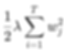
Within the regularization term, we have γT, where:
T = number of leaf nodes in the decision tree.
γ (gamma) = regularization parameter that penalizes the number of leaf nodes.
This means the γT term discourages the model from creating too many leaf nodes. If a tree has too many leaves, it becomes highly complex and risks overfitting. By penalizing leaf growth, gamma helps in:
Reducing unnecessary leaf nodes.
Controlling model complexity.
Acting as a form of post-pruning, since it prunes trees after they are formed.
In short, a higher value of gamma (γ) makes the algorithm more conservative by preventing excessive tree splitting, thus improving generalization.
Suppose we already have:
m1 = mean model,
m2 = first decision tree,
m3 = second decision tree,
and now we want to add m4, the third decision tree.
In XGBoost, splitting is done on the basis of the similarity score (SS).
When a node is split, we calculate the similarity scores for its left and right child nodes.
The gain is then computed as:

This measures the improvement achieved by splitting a node.
On strict mathematical form, the gain is written as:

Here, γ (gamma) acts as a pruning parameter.
Example with Node Values
Assume we have nodes with similarity scores 1200, 600, 300.
These values represent similarity scores, not gains at leaf nodes.
We calculate gains only for splits, not for leaf nodes (for leaves, we only record similarity scores).
Using Gamma (γ) for Pruning
To perform pruning, we set a value of γ.
If Gain – γ > 0, we keep the split (the node is useful).
If Gain – γ ≤ 0, we prune (remove) the split.
Case 1: γ = 100
Node with gain = 300 → 300 − 100 = 200 > 0 → keep
Node with gain = 600 → 600 − 100 = 500 > 0 → keep
Node with gain = 1200 → 1200 − 100 = 1100 > 0 → keep
All nodes are kept, so no pruning happens.
Case 2: γ = 800
Node with gain = 300 → 300 − 800 = −500 < 0 → prune
Node with gain = 600 → 600 − 800 = −200 < 0 → prune
Node with gain = 1200 → 1200 − 800 = 400 > 0 → keep
Only the root node (1200) is kept, and smaller branches are pruned.
Key Idea
Gamma (γ) acts as a threshold for pruning.
A small γ → more splits, complex trees, higher risk of overfitting.
A large γ → fewer splits, simpler trees, better generalization.
This is how post-pruning is applied in XGBoost using the gain formula.
Special Case in Post-Pruning with Gamma (γ)
Consider the following decision tree with gains:
Root node = 1200
Left child = 300
Right child = 600
Case: γ = 500
Node with gain = 600
600 − 500 = 100 > 0
Since the result is positive, this split is kept.
Node with gain = 300
300 − 500 = −200 < 0
Because the result is negative, this split is pruned.
Important correction: In XGBoost, a node cannot be kept just because its child has a higher gain. Each node is evaluated independently against γ.
Root node with gain = 1200
1200 − 500 = 700 > 0
The root is also kept.
In this case, pruning occurred on the left branch (gain = 300), while the right branch and root were preserved.
Key Insights
Gamma (γ) acts as a threshold on gain.
If Gain < γ, the node is pruned.
If Gain ≥ γ, the node is kept.
Why this matters:
γ prevents the tree from growing too complex.
It acts as a tunable threshold for model complexity.
Choosing γ:
There is no fixed rule — it must be tuned experimentally.
γ = 0 → allows maximum splits → risk of overfitting.
Large γ → aggressive pruning → risk of underfitting.
The beauty of γ is that it provides flexibility in controlling complexity. By adjusting γ, we balance between overfitting (too many splits) and underfitting (too few splits).
XGBoost Parameter: Max Depth
Definition:
max_depth sets the maximum depth of decision trees in XGBoost.
No tree is allowed to grow deeper than this limit.
It is a form of pre-pruning (restriction applied before tree growth).
Why Max Depth?
You may wonder: “If gamma already prunes trees, why do we need max depth?”
The answer is computation efficiency:
If max_depth = None, the tree grows fully, and then gamma/post-pruning trims it.
This means wasted computation → building branches that will eventually be removed.
By setting a max depth early, we avoid unnecessary splits and reduce training cost.
In short:
Gamma → post-pruning (after tree growth).
Max Depth → pre-pruning (limits growth upfront).
Practical Insight
Shallow trees (small depth) → underfitting (too simple).
Very deep trees → overfitting (too complex).
Common range: 3 to 10 for tabular problems, but depends on dataset size & complexity.
Max Depth = computation control + complexity control.
It prevents the model from growing unnecessarily deep trees and balances efficiency with generalization.
XGBoost Parameter: min_child_weight
What it Does
min_child_weight is a regularization parameter that helps in pruning decision trees, making them simpler and reducing overfitting.
To understand it, we first need to understand the concept of cover.
Cover (Sum of Hessians)
In boosting, every node has a cover, which is the sum of Hessians at that node.
Hessian (hᵢ): The second derivative of the loss function (differentiation of the gradient).
Gradients and Hessians are used in computing similarity scores, gain, and leaf values in XGBoost.
Formally:
Regression: hᵢ = 1 for all data points.
Classification: hᵢ = pᵢ(1-pᵢ) , where pᵢ is the probability from the previous stage.
Thus:
Cover = Σ hᵢ (sum of Hessians at a node).
Interpretation of Cover
Regression: Since hᵢ = 1, cover = number of data points at that node.
Classification: Cover = sum of pᵢ(1-pᵢ) .
If pᵢ is close to 0 or 1 → hᵢ is small → point is already “easy to classify”.
If pᵢ ≈ 0.5 → hᵢ is large (max 0.25) → model is uncertain → point is “important”.
Cover therefore quantifies how important data points at a node are for further splitting.
How min_child_weight Works
Splitting at a node happens only if cover ≥ min_child_weight.
If cover < min_child_weight → the node will not split (pruned).
This is similar to min_samples_split in Decision Trees.
Regression case: min_child_weight behaves like a minimum sample requirement (since cover = number of points).
Classification case: It ensures splits only when the sum of Hessians (importance of uncertain points) is large enough.
Example: Classification Case
Suppose we have data:
cgpa | placement | pred | res | pred2 | res2 |
8 | 1 | 0.5 | 0.5 | 0.7 | 0.3 |
7 | 0 | 0.5 | -0.5 | 0.3 | -0.3 |
4 | 0 | 0.5 | -0.5 | 0.2 | -0.2 |
5 | 1 | 0.5 | 0.5 | 0.8 | 0.2 |
For classification, Hessians are:
hᵢ = pᵢ(1-pᵢ)
If p = 0.7 → h = 0.21
If p = 0.3 → h = 0.21
If p = 0.2 → h = 0.16
If p = 0.8 → h = 0.16
So, cover = sum of Hessians = 0.21 + 0.21 + 0.16 + 0.16 = 0.74
If min_child_weight = 1 → split won’t happen because cover < 1.
If min_child_weight = 0.5 → split is allowed.
Intuition
High Hessian → model is uncertain about the prediction (important to split).
Low Hessian → model is confident (not important to split).
By setting min_child_weight, we control which nodes are allowed to split.
Key Insights
Large min_child_weight → fewer splits → simpler model → may underfit.
Small min_child_weight → more splits → complex model → may overfit.
min_child_weight ensures that a node only splits when there are enough important (uncertain) data points, preventing the model from learning noise.
Number of Estimators (n_estimators)
The parameter n_estimators in XGBoost controls the number of boosting rounds (trees) used to build the model.
If n_estimators is too large, the model may become too complex, increasing the risk of overfitting.
If n_estimators is too small, the model may be too simple, leading to underfitting.
The key is to balance the number of trees so the model generalizes well to unseen data.
Early Stopping
Boosting works by adding models iteratively:
Model 1 makes predictions → errors are calculated.
Model 2 is trained to fix the errors of Model 1.
Model 3 is trained on errors of Model 2, and so on.
But when should we stop adding more trees?
If we keep adding trees without stopping:
Training loss will continue to decrease (the model fits training data better and better).
Test/validation loss will first decrease, then start increasing when the model begins overfitting.
Visualization (Loss vs. Number of Trees)
X-axis: Number of trees (n_estimators).
Y-axis: Loss (training loss & test/validation loss).
At the beginning → both training and test loss are high.
As trees are added → both losses decrease.
After a certain point → training loss keeps decreasing, but test loss starts increasing → overfitting begins.
The best stopping point is where test loss is minimal.

How Early Stopping Works
We define a patience value (e.g., early_stopping_rounds = 10).
During training, XGBoost monitors validation loss:
If the loss doesn’t improve for 10 consecutive rounds, training stops.
The model then uses the best iteration (the one with minimum validation loss).
This prevents wasting computation on unnecessary trees and helps avoid overfitting.
In summary:
n_estimators decides how many boosting rounds to run.
early_stopping automatically finds the best point to stop before overfitting begins.
6. Shrinkage / Learning Rate
Definition:
The learning rate (also called shrinkage) scales the contribution of each new tree before it is added to the model.
Instead of fully trusting each tree, we multiply its predictions by the learning rate (a fraction).
This ensures the model learns in smaller, controlled steps.
Intuition
Imagine the “perfect solution” is 5.23.
Without a learning rate (LR = 1):
The model jumps in whole steps → 1, 2, 3, 4, 5, 6 …
→ It overshoots and misses the precise value 5.23.
With a smaller learning rate (say LR = 0.1):
Each step is smaller → 1, 1.1, 1.2, …, 5.1, 5.2, 5.3 …
→ Now we can get much closer to 5.23.
With an even smaller learning rate (say LR = 0.01):
The steps are very fine → 1, 1.01, 1.02 …, 5.01, 5.02 …, 5.23
→ We can exactly approach the target but at the cost of needing many more trees.
So, the learning rate balances precision vs. speed in reaching the optimal solution.
Key Trade-offs
High learning rate →
Fast learning but risks overshooting the optimal solution.
May converge quickly but can miss the best model.
Low learning rate →
Very precise but requires many trees → slower, more computationally expensive.
Safer against overfitting but less efficient.
Practical Tip
Default (and widely used) value: 0.3.
Often combined with a higher n_estimators to compensate for smaller steps.
In practice, smaller LR (0.01–0.1) + more trees usually gives the best results.
In short:
Learning rate makes boosting gradual and controlled.
Too high → risk missing the optimum.
Too low → too slow.
The sweet spot is chosen by experimentation + validation.
Lambda (reg_lambda)
Definition:
In XGBoost, the objective function has two parts:
Loss function – measures how well predictions fit actual values.
Regularization term – prevents overfitting by penalizing complexity.
The regularization term includes λ (lambda):

T = number of leaf nodes
wⱼ = weight/output value of each leaf
This is essentially L2 regularization.
How Lambda Works
In Similarity Score

If λ increases → denominator increases → similarity decreases.
Lower similarity → lower gain → more pruning.
In Gain Formula

Gain decreases as λ increases.
If Gain < Gamma → prune that node.
Thus, larger λ indirectly increases pruning, leading to simpler trees.
In Leaf Output Calculation

If λ increases → leaf values shrink → smaller outputs.
This behaves like a shrinkage effect, similar to learning rate (but applied at the leaf level).
Effects of Lambda
Increase λ →
Gain ↓
Similarity score ↓
Leaf output values ↓
More pruning → simpler trees → less overfitting
Risk: underfitting if λ too high
Decrease λ →
Gain ↑
Leaf outputs ↑
Complex trees → risk of overfitting
Connection with Gamma
Gamma (γ) → explicit pruning threshold (node is pruned if Gain < Gamma).
Lambda (λ) → reduces Gain values → indirectly increases pruning chance.
Together: λ lowers Gain, γ decides cutoff → both work hand in hand.
Regularization Types
reg_lambda (λ): L2 Regularization
→ Makes leaf outputs smaller, smoother.
reg_alpha (α): L1 Regularization

→ Drives some leaf outputs exactly to zero → feature selection effect.
Elastic Net (α + λ):
→ Combines L1 + L2.
Lambda reduces leaf values & gain → simpler trees → less overfitting.
Works like shrinkage + pruning helper.
L2 (λ) is more common than L1 (α), but both can be combined (Elastic Net).
Subsample
Definition:
Similar to Random Forest, XGBoost can train each tree on a random subset of rows from the training data instead of the full dataset.
Parameter range: 0 < subsample ≤ 1
How It Works
If subsample = 1.0: each tree sees the full dataset.
If subsample = 0.5: each tree is trained on a random 50% of rows.
Example:
Dataset has 100 rows.
Tree 1 trained on random 50 rows.
Tree 2 trained on another random 50 rows.
…and so on.
This creates randomness → different trees learn different perspectives.
Effect on Model
Helps reduce overfitting (trees don’t all see identical data).
Too low value (<0.5) → underfitting (not enough information per tree).
Too high (≈1.0) → trees too similar → overfitting.
Good range: 0.5 – 0.8
Intuition
This is “wisdom of the crowd.”
Different subsets of data → different decisions → ensemble combines them → stronger generalization.
Colsample (Column Subsampling)
Definition:
Instead of giving all features (columns) to every tree, we can give only a random subset of features.
This introduces more randomness and makes trees more diverse.
Types:
colsample_bytree
Selects a random subset of features once per tree.
Example: If 10 features and colsample_bytree = 0.5, then randomly select 5 features, and the whole tree is built using only those 5.
colsample_bylevel
Randomly selects a subset of features at each level of the tree.
Example: At root node, pick 5 features; at next level, pick a new random 5, etc.
Creates more randomness than bytree.
colsample_bynode
Randomly selects a subset of features at each split (node).
Example: At every node, choose 5 random features for that split.
This introduces the highest randomness among the three.
Effect on Model
Reduces overfitting by preventing trees from always using the strongest features.
Ensures the model explores different “views” of the data.
Works very well when you have many features.
Summary
Subsample (rows): controls how many data samples each tree sees.
Colsample (columns): controls how many features each tree/level/node sees.
Together, they create diversity → reduce overfitting → improve generalization.