Backpropagation Through Time (BPTT) Explained Step-by-Step with a Simple RNN Example

To understand how RNNs learn, let's walk through the process using a simple "toy" dataset. We will look at data preparation, the architecture, and the forward propagation steps that lead into calculating gradients.

Data Preparation

We start with a dataset consisting of just three reviews. Our entire vocabulary consists of only three unique words: cat, mat, rat.

The Reviews & Sentiment Labels:

• Review 1: "cat mat rat" → Positive Sentiment (1)

• Review 2: "rat rat mat" → Positive Sentiment (1)

• Review 3: "mat mat cat" → Negative Sentiment (0)

To feed this into our network, we convert each word into a vector using One-Hot Encoding. Since our vocabulary size is 3, each word is represented by a 3-dimensional vector:

• cat: [1, 0, 0]

• mat: [0, 1, 0]

• rat: [0, 0, 1]

Vectorized Input (X) vs. Target (Y):

Input Sequence (X)	Sequence ID	Label (Y)
[100], [010], [001]	X₁	1
[001], [001], [010]	X₂	1
[010], [010], [100]	X₃	0

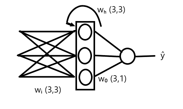
The RNN Architecture

Now, let's define the architecture we are feeding this data into. We will assume a standard RNN structure with the following specifications:

• Input Layer: Receives 3-dimensional vectors (one word at a time).

• Hidden Layer: Contains 3 neurons. This layer maintains the "memory" of the sequence.

• Output Layer: Contains 1 node (since this is a binary classification task).

The Parameters (Weights):

To process the data, our network learns three specific weight matrices:

1. Wᵢ (Input-to-Hidden): Weights connecting the input vector to the hidden layer. Shape: (3, 3).

2. Wₕ (Hidden-to-Hidden): Weights connecting the previous hidden state to the current hidden state (the recurrent component). Shape: (3, 3).

3. Wₒ (Hidden-to-Output): Weights connecting the final hidden state to the output node. Shape: (3, 1).

   

Forward Propagation Through Time

Forward propagation in an RNN works by unfolding the network across time steps. We process a single review (sequence) word by word.

Let's trace the first review (X₁ : "cat mat rat") through the network:

1. Time Step 1: We input "cat" (100). The network computes the first hidden state, O₁ .

2. Time Step 2: We input "mat" (010). The network uses the current input and the previous state O₁ to compute O₂.

3. Time Step 3: We input "rat" (001). The network uses the input and O₂ to compute O₃.

Since there are no more words, O₃ is our final hidden state. We pass this into the output layer to get our final prediction.

The Forward Propagation Equations:

Mathematically, the calculations at each step look like this:

O₁ = f(x₁₁Wᵢ + O₀Wₕ)

O₂ = f(x₁₂Wᵢ + O₁Wₕ)

O₃ = f(x₁₃Wᵢ + O₂Wₕ)

Finally, the prediction ŷ is generated using the activation function (like Sigmoid) on the final state:

ŷ = σ(O₃W₀)

Loss Calculation & Backpropagation

Once we have the prediction ŷ and the true label y, we calculate the error using the Binary Cross Entropy loss function:

L = - yᵢ log(ŷᵢ) - (1 - yᵢ) log(1 - ŷᵢ)

Minimizing Loss:

Our goal is to find the optimal values for Wᵢ, Wₕ, and Wₒ that minimize this loss. We achieve this using Gradient Descent. We calculate the derivative of the Loss (L) with respect to each weight matrix and update them:

(Where η is the learning rate)

By repeating this process—forward passing the data, calculating loss, and backpropagating the errors to update weights—our RNN learns to classify the sentiment of the reviews correctly.

Calculating Derivatives (The Backward Pass)

We have initialized our weights and defined our forward pass equations. Now, to minimize the loss, we need to find the derivative of the Loss function (L) with respect to each of our weight matrices (Wₒ, Wᵢ, Wₕ).

Let's recall our forward pass equations for the three time steps:

A. Derivative with respect to Output Weights (Wₒ)

This is the most straightforward derivative. If we change Wₒ, it directly affects the prediction ŷ, which changes the Loss L.

Since Wₒ only appears at the final stage (connected to O₃), there is only one path to trace.

Using the chain rule:

We calculate this using our loss equation and update Wₒ directly.

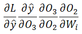
B. Derivative with respect to Input Weights (Wᵢ)

Calculating the derivative for Wᵢ is trickier. Why? Because the weight matrix Wᵢ is shared across all time steps. It was used to calculate O₁, then used again for O₂, and again for O₃.

If we look at the dependency chain:

1. L depends on ŷ.

2. ŷ depends on O₃.

3. O₃ depends on O₂ AND Wᵢ.

4. O₂ depends on O₁ AND Wᵢ.

5. O₁ depends on Wᵢ.

Because Wᵢ contributed to the error at three different points in time, we have to sum up the gradients from all three paths.

The Three Paths:

1. Direct Path (Time 3): L → ŷ → O₃ → Wᵢ

2. Path through O₂ (Time 2): L → ŷ → O₃ → O₂ → Wᵢ

3. Path through O₁ (Time 1): L → ŷ → O₃ → O₂ → O₁ → Wᵢ

The Expanded Equation:

We add these paths together to get the total derivative:

Writing this out for long sequences (like 10 or 100 words) is very hard, so we summarize it using summation notation.

The General Formula:

(Where n is the number of time steps. In our case, n = 3.)

For example, for timestep j = 1:

Since ŷ​ depends on O₃​, the chain expands as:

Substituting gives:

Similarly, for j = 2:

And for j = 3:

Combining all terms gives the final backpropagation-through-time expression:

where n is the number of timesteps.

C. Derivative with respect to Recurrent Weights (Wₕ)

The logic for Wₕ is identical to Wᵢ. Since Wₕ is the weight connecting hidden states (O₀ → O₁ → O₂ → O₃), it is also responsible for carrying information through time.

Just like before, we have three paths because Wₕ was used three times. We must account for the non-linear relationship where the current state depends on the previous one.

The Expanded Equation:

The General Formula:

The Gradient Descent Cycle

Now that we have the formulas for the three required derivatives

we apply the Gradient Descent algorithm to train our model.

1. Initialize random weights and a learning rate.

2. Forward Pass: Take a review, feed it word-by-word, calculate hidden states (O₁, O₂, O₃), and get the final prediction.

3. Calculate Loss: Compare prediction with the true label.

4. Backward Pass (BPTT): Calculate the derivatives using the summation formulas derived above. This "unfolds" the network back through time to account for shared weights.

5. Update Weights:

   

6. Repeat: We do this constantly for all reviews until the loss is minimized and the parameters reach their optimal values.