
DECISION TREES - 2
- Aryan

- May 17, 2025
- 9 min read
Decision Trees for Regression (CART)
Let’s explore how CART (Classification and Regression Trees) works for regression tasks using the sample dataset below :
Subject | Grade_Level | Hours_Studied | Test_Score |
Math | Freshman | 4 | 59 |
Physics | Freshman | 1 | 82 |
Physics | Freshman | 4 | 81 |
Math | Junior | 6 | 60 |
Physics | Sophomore | 1 | 73 |
Physics | Junior | 3 | 85 |
Physics | Junior | 4 | 61 |
Physics | Freshman | 9 | 78 |
Key Concepts
The dataset contains categorical (Subject, Grade_Level) and numerical (Hours_Studied) input features.
The target variable is Test_Score, which is continuous, so we use CART for regression, not classification.
How CART Works for Regression
In classification tasks, CART uses Gini impurity to decide the best feature and threshold for splitting the data.
But for regression, we replace Gini impurity with Mean Squared Error (MSE) or variance.
Our goal is to reduce variance in the target variable (Test_Score) after each split.
What does CART try to do?
Try all features and all possible splits.
For each split, calculate the weighted MSE of the two resulting groups.
Choose the split that gives the maximum reduction in MSE (or minimum weighted MSE).
This becomes the root node.
The process repeats recursively on each branch.
Example Intuition
Let’s say we try a split like :
Hours_Studied <= 4
CART will :
Divide the dataset into two parts :
Group A (Hours_Studied <= 4) and Group B (Hours_Studied > 4)
Compute variance or MSE of Test_Score in each group
Compute weighted average of these variances
Compare it to other possible splits (e.g., by Subject or Grade_Level)
The split that reduces the overall variance the most becomes the decision point .
In short :
For regression, CART chooses the feature and threshold that lead to the greatest reduction in variance in the target variable.
Computing the Split MSE for Subject = Math
Continuing our CART‐for‐regression example, let’s evaluate the candidate split:
“Subject == Math?”
– Yes (Math) group
– No (Physics) group
We want to compute the weighted mean squared error (MSE) of the two groups, then compare it to other splits.
Partition the data
Subject | Test_Score |
Yes (Math) | 59, 60 |
No (Physics) | 82, 81, 73, 85, 61, 78 |
Size_yes = 2
Size_no = 6
Total = 8
Compute each group’s mean

Compute each group’s MSE

Compute the weighted MSE (overall impurity) of the split

Interpretation :
Splitting on Subject = Math yields a weighted MSE of ≈ 47.24.
In CART for regression, we would compare this value against the MSEs from other possible splits (e.g. Hours_Studied ≤ t or different Grade_Level splits) and choose whichever split minimizes the weighted MSE.
Evaluating Splits on Grade_Level
Our goal is to treat Grade_Level (with categories Freshman, Junior, Sophomore) as a candidate split, and compute the weighted variance (MSE) for each of the three possible binary partitions:
Freshman vs {Junior, Sophomore}
Junior vs {Freshman, Sophomore}
Sophomore vs {Freshman, Junior}
Whichever split yields the lowest weighted variance becomes our choice for the root node on Grade_Level .
Data Recap
Index | Grade_Level | Test_Score |
0 | Freshman | 59 |
1 | Freshman | 82 |
2 | Freshman | 81 |
3 | Junior | 60 |
4 | Sophomore | 73 |
5 | Junior | 85 |
6 | Junior | 61 |
7 | Freshman | 78 |
Total n = 8 observations.
Split A: Freshman vs {Junior, Sophomore}

Split B: Junior vs {Freshman, Sophomore}

Split C: Sophomore vs {Freshman, Junior}

Choosing the Best Split
Split Option | Weighted MSE |
Freshman vs {Junior, Sophomore} | 95.59 |
Junior vs {Freshman, Sophomore} | 94.23 |
Sophomore vs {Freshman, Junior} | 102.43 |
Result: The lowest weighted variance is 94.23, achieved by the split
Grade_Level == Junior
Hence, “Is Grade_Level = Junior?” becomes our optimal decision at this node.
Evaluating Splits on Hours_Studied
To include our continuous feature Hours_Studied, we consider all possible mid‐point thresholds and compute the weighted MSE for each :
Sorted Hours | 1, 1, 3, 4, 4, 4, 6, 9 |
Mid‐points | (1+3)/2 = 2, (3+4)/2 = 3.5, (4+6)/2 = 5, (6+9)/2 = 7.5 |
For each threshold t , we split :
Yes : Hours_Studied > t
No : Hours_Studied ≤ t
and compute

Split at t = 2

Split at t = 3.5

Split at t = 5

Split at t = 7.5

Best Hours_Studied Split
Threshold t | Weighted MSE |
2 | 93.64 |
3.5 | 67.88 |
5 | 98.69 |
7.5 | 97.74 |
The lowest MSE is 67.88 at Hours_Studied > 3.5
Choosing the Root Node
Recall our previous root‐split MSEs :
Feature Split | MSE |
Subject = Math | 47.24 |
Grade_Level = Junior | 94.23 |
Hours_Studied > 3.5 | 67.88 |
Winner:
Subject = Math has the lowest MSE (47.24) , so it becomes the root node of our regression tree.
GEOMETRIC INTUITION
In classification problems, decision trees operate by recursively splitting the dataset based on feature values. These splits occur along the coordinate axes (i.e., axis-aligned hyperplanes), dividing the feature space into distinct decision regions—for example, one region for red-labeled points and another for green-labeled points.
Suppose there is a green point mistakenly placed in a red-dominated region. To correctly classify it, the decision tree will introduce additional axis-aligned splits around that point, creating a new, isolated sub-region. This process continues for other such points, as the tree attempts to perfectly classify all training examples.

As a result, the decision boundary becomes highly fragmented, with the entire feature space divided into many small and irregular regions. This behavior leads to overfitting, where the model captures noise and outliers in the training data instead of generalizable patterns.
Because of this tendency to split excessively and form overly complex regions, decision trees are highly prone to overfitting, especially when not pruned or regularized properly. This geometric intuition explains why decision trees often need techniques like pruning, depth limitation, or ensemble methods (e.g., Random Forests) to improve generalization.

Geometric Intuition Behind Decision Trees for Regression
Decision trees are intuitive and powerful models for both classification and regression tasks. In regression, the goal is to predict a continuous output variable, and decision trees do this by splitting the input space into regions where a constant prediction (typically the mean of target values) is made.
Let’s understand this process geometrically and intuitively, using a real-world-inspired example : predicting a student’s exam score based on their study hours .
Dataset Example
We’ll work with a small, illustrative dataset :
Study Hours | Exam Score |
1 | 30 |
3 | 50 |
6 | 80 |
8 | 60 |
10 | 40 |
We intentionally chose a dataset with non-linear behavior. You’ll notice that :
At very low hours (1), score is low (30).
Around mid-range hours (6), score is high (80).
At high hours (10), score drops again (40).
This suggests a non-linear relationship. A linear regression model would fail here, but decision trees are well-suited due to their piecewise constant approximation ability.
How Decision Trees Work in Regression
The tree recursively divides the input space (in our case, "study hours") into segments where the output (exam score) is more "homogeneous", i.e., has lower variance. The criterion for choosing a split is typically to minimize the total variance after the split.
Let's see this step-by-step.
Step 1 : Visualizing the Raw Dataset

This scatter plot shows the non-linear pattern clearly .
Step 2 : One Split (Creating Two Regions)
Let’s attempt our first split at Hour = 5. This divides the data into :
Left Region (Hours ≤ 5) → Points: (1, 30), (3, 50)
Right Region (Hours > 5) → Points: (6, 80), (8, 60), (10, 40)
Each region now predicts the average score of its data points :
Left prediction: (30+50)/2 = 40
Right prediction: (80+60+40)/3 = 60
This is our first piecewise constant model .

Observation:
We now have two regions, each predicting a flat constant value. The total variance within each region is reduced compared to the full dataset.
Step 3: Two Splits (Creating Three Regions)
Let’s now split further — this time, we add a second split at Hour = 7.
Now, we have :
Region 1 : Hours ≤ 5 → (1, 3) : Avg = 40
Region 2 : 5 < Hours ≤ 7 → (6) : Avg = 80
Region 3 : Hours > 7 → (8, 10) : Avg = (60+40)/2 = 50

Observation:
The model is more flexible now. It adapts better to the rise and fall in scores, and the variance within regions is even lower.
Step 4: Overfitting — Splitting at Every Data Point
Let’s now push the model to its extreme. If we split at every input point, we end up with five tiny regions, each holding one data point.
Now each region’s prediction is just the actual score of the single data point it contains. This leads to a model with zero training error, but it's extremely fragile and will likely fail on unseen data.

What’s the Problem ?
The model memorizes the data instead of learning a general pattern.
It has zero bias (perfect on training set), but very high variance (sensitive to noise and new points).
This is a textbook example of overfitting.
The Geometry of It All
Visually, decision trees for regression create a staircase-like function. Each step is a constant value prediction in a region. More steps = more flexibility = better fit on training data… but eventually, you create a function that’s jagged and brittle.
Recap : Bias-Variance Tradeoff in Tree Splits
Split Strategy | Description | Bias | Variance | Generalization |
No Split (1 region) | Predict global mean | High | Low | Poor |
Few Splits | General pattern with some error | Medium | Medium | Good |
Many Splits | Fit every data point | Low | High | Poor |
Final Thought
This geometric walkthrough shows how decision trees carve the input space into axis-aligned regions. Each region holds a simple prediction, but too many regions cause the model to lose generalization.
Always control model complexity to balance fit and flexibility.
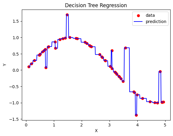
HOW PREDICTION IS DONE (REGRESSION TREE)

The diagram above represents a regression decision tree where we have one input feature x and one output y. The tree recursively splits the data into regions using thresholds on the feature values. These thresholds are visible as vertical lines in the second image, which show how the feature space is partitioned.
Let’s consider a new data point :
x = 2.9
We use the decision tree to predict its corresponding y value as follows:
Start at the root node:
Condition : x[0] <= 3.724
Since 2.9 <= 3.724 is True, we follow the left branch.
At the next node:
Condition : x[0] <= 2.792
Since 2.9 <= 2.792 is False, we follow the right branch.
We reach a leaf node with a value of 0.059.
Hence, the predicted y value for x = 2.9 is : 0.059
WHY THE OUTPUT IS 0.059
This output is determined by the region where the input falls after the tree’s splits. The value 0.059 is the mean (average) of the target y values for all training data points that fall into that region (i.e., the same leaf node).

The second image illustrates this geometrically :
The input space has been divided into four regions by three vertical splits at x = 2.792, x = 3.724, and x = 3.925.
Each region contains data points, and the average y value of points in each region is stored at the corresponding leaf node of the tree.
These leaf values are what the model uses to make predictions.
GENERAL CASE
If the decision tree is deeper or the input has more features :
There will be more splits and more leaf nodes.
The new input will traverse the tree based on the conditions at each node.
Once it reaches a leaf node, the predicted output is the average y value of the training points in that leaf's region.
This is the essence of how regression using decision trees makes predictions.
HOW PREDICTION IS DONE (CLASSIFICATION TREE)
In the case of classification, decision trees are used to predict categorical labels (e.g., species of a flower). Let’s understand how prediction works using an example .

Suppose we have a decision tree trained on the Iris dataset using two input features:
Sepal length
Sepal width
The goal is to classify a flower into one of the three species :
Setosa, Versicolor, or Virginica.
Example 1 : Predict for Input {4.9, 3}
Step 1 (Root Node) :
Condition : sepal length <= 5.45
Input: 4.9 → True → go to the left child.
Step 2 :
Condition : sepal width <= 2.8
Input : 3.0 → False → go to the right child.
Leaf Node :
The predicted class here is Setosa.
Prediction : Setosa
Example 2: Predict for Input {6.0, 2.0}
Step 1 (Root Node) :
Condition : sepal length <= 5.45
Input : 6.0 → False → go to the right child.
Step 2 :
Condition : sepal length <= 6.15
Input : 6.0 → True → go to the left child.
Leaf Node :
The predicted class here is Versicolor.
Prediction : Versicolor
HOW CLASSIFICATION OUTPUT IS DECIDED
In regression trees, the output is a mean of target values in the region.
But in classification trees, the output is determined by a majority vote among the training samples in that leaf node:
Each leaf node contains samples from one or more classes.
The class with the highest count becomes the predicted label.
This is known as the majority class in that region.
Advantages
Simple to understand and to interpret. Trees can be visualized.
Requires little data preparation. Other techniques often require data normalization, dummy variables need to be created and blank values to be removed. Note however that this module does not support missing values.
The cost of using the tree (i.e., predicting data) is logarithmic in the number of data points used to train the tree.
Able to handle both numerical and categorical data.
Can work on non-linear datasets.
Can give you feature importance.
Disadvantages
Decision-tree learners can create over-complex trees that do not generalize the data well. This is called overfitting. Mechanisms such as pruning, setting the minimum number of samples required at a leaf node or setting the maximum depth of the tree are necessary to avoid this problem.
Decision trees can be unstable because small variations in the data might result in a completely different tree being generated. This problem is mitigated by using decision trees within an ensemble.
Predictions of decision trees are neither smooth nor continuous, but piecewise constant approximations as seen in the above figure. Therefore, they are not good at extrapolation. This limitation is inherent to the structure of decision tree models. They are very useful for interpretability and for handling non-linear relationships within the range of the training data, but they aren't designed for extrapolation. If extrapolation is important for your task, you might need to consider other types of models.


