Encoder–Decoder (Seq2Seq) Architecture Explained: Training, Backpropagation, and Prediction in NLP

SEQ2SEQ DATA

The first major challenge in machine learning came with tabular data, where traditional algorithms and later Artificial Neural Networks (ANNs) were sufficient. As image data emerged, a new problem appeared. Images are composed of pixels, which form a two-dimensional grid of data. This spatial structure carries meaning that standard ANNs could not effectively capture, which led to the development of Convolutional Neural Networks (CNNs).

The next challenge was sequential data, where the order of data points matters. Examples include textual data and time-series data. In such cases, the sequence itself carries information. ANNs and CNNs are not designed to model temporal dependencies, so Recurrent Neural Networks (RNNs) were introduced, followed by improved variants such as LSTM and GRU to handle long-term dependencies.

Now we face a fourth and more complex challenge: sequence-to-sequence (seq2seq) data. In this type of problem, both the input and the output are sequences. A classic example is machine translation. Suppose we have an English sentence, “nice to meet you,” and we want to translate it into Hindi, producing “aapse milkar achha laga.” Here, both input and output are sequences.

Sequence-to-sequence problems are difficult due to three key challenges. First, the input sentence has a variable length. Second, the output sentence also has a variable length. Third, there is no guarantee that the input and output sequences will have the same length. For example, a three-word English sentence may translate into a Hindi sentence with more or fewer words. Handling this variability in both input and output length is the core difficulty.

While LSTM and GRU can handle variable-length input sequences, we also need a mechanism to generate variable-length outputs. To address this, we study the encoder–decoder architecture, using machine translation as a guiding example.

HIGH-LEVEL OVERVIEW

The encoder–decoder architecture consists of two main blocks: an encoder and a decoder. These two blocks are connected through a vector known as the context vector.

The encoder is responsible for processing the input sequence. The input sentence is fed to the encoder token by token (or word by word). As the encoder processes the sequence, it tries to capture the overall meaning or essence of the sentence. After processing the final token, the encoder produces a fixed-length numerical representation called the context vector. This vector is essentially a summary of the entire input sequence.

The decoder takes this context vector as input and generates the output sequence one token at a time. Using the information stored in the context vector, the decoder predicts the output tokens sequentially until the full translated sentence is produced.

In simple terms, the encoder understands and summarizes the input, and the decoder uses that summary to generate the output sequence step by step. This forms the high-level working of the encoder–decoder architecture.

WHAT’S UNDER THE HOOD ?

Both the encoder and the decoder must be capable of processing sequential data. For this reason, LSTMs are commonly used in both components, although GRUs can also be used.

The encoder is essentially a single LSTM cell unfolded over time. At each time step, one input token is fed into the LSTM. Initially, the hidden state hₜ​ and cell state cₜ​ are initialized, often with zeros or random values. As each word (for example, “nice,” then “to,” then “meet,” then “you”) is processed, the LSTM updates its hidden and cell states. Through this process, the LSTM gradually captures the semantic information of the entire sentence.

After the final time step, the encoder’s last hidden state and cell state represent the final summary of the input sequence. This final representation is referred to as the context vector and is passed to the decoder. In summary, the encoder converts a variable-length input sequence into a fixed-length representation.

The decoder also uses an LSTM, but it is a separate network with its own parameters. Its job is to generate an output token at each time step. The initial hidden and cell states of the decoder are typically set to the final hidden and cell states of the encoder. At the first time step, the decoder is given a special <START> token along with the context information, and it generates the first output token.

At each subsequent time step, the decoder takes the previously generated token as input, along with the updated hidden and cell states, and produces the next token. This process continues until a special <END> token is generated. Once the decoder outputs the end token, it stops generating further tokens.

This step-by-step generation mechanism allows the decoder to produce output sequences of variable length, which is exactly what is required for sequence-to-sequence tasks such as machine translation.

TRAINING THE ENCODER–DECODER ARCHITECTURE USING BACKPROPAGATION

Now we will understand how the encoder–decoder architecture is trained using backpropagation. We will take machine translation as an example. The datasets used for this task are called parallel datasets. Each data point contains two features: the input sentence in one language (English) and its corresponding translated sentence in another language (Hindi).

For example, our dataset may look like this:

Eng	Hindi
Think about it	Soch lo
Come in	Andar aa jao

 To train the encoder–decoder model, we feed this paired data into the network. However, the problem is that the dataset is in natural language, and neural networks cannot directly process words or text. Therefore, the first step is to convert the text into numerical form.

We begin with tokenization, where each sentence is split into individual tokens (words). After tokenization, the data looks like:

[think, about, it] → [soch, lo]

[come, in] → [andar, aa jao]

Next, we apply one-hot encoding. Suppose our English vocabulary consists of five unique words. Each word is represented as a vector of length five, where only one position is set to 1 and the rest are 0. For example:

Think → [1, 0, 0, 0, 0]

About → [0, 1, 0, 0, 0]

We perform a similar encoding for Hindi words. However, for the output language, we also introduce two special tokens: <START> and <END>. These tokens help the decoder understand when to begin and stop generating output. After including these tokens, suppose the Hindi vocabulary size becomes seven. The encoding may look like:

<START> → [1, 0, 0, 0, 0, 0, 0]

soch → [0, 1, 0, 0, 0, 0, 0]

Now both input and output sequences are in numerical form, and we can pass them through the architecture. We start with the first training example:

think about it → soch lo

The encoder and decoder each contain their own LSTM networks. These are separate LSTMs with independently initialized weights and biases. Initially, all parameters are randomly initialized.

At the first time step, the encoder receives the word think encoded as [1, 0, 0, 0, 0], along with initial hidden state h₀ and cell state c₀ ​. The LSTM processes this input and produces updated hidden and cell states. At the next time step, the word about is passed, followed by it. Across these three time steps, the encoder gradually updates its internal states to capture the meaning of the entire sentence.

After the final time step, the encoder outputs its final hidden state and cell state. Together, these represent the context vector, which is a compressed representation of the input sentence. This context vector is passed to the decoder.

The decoder LSTM uses the encoder’s final hidden and cell states as its initial states. At the first decoder time step, we provide the <START> token as input. The decoder produces an output vector, but since neural networks output numbers, not words, we use a softmax layer to convert this output into probabilities over the output vocabulary.

The softmax layer has one neuron for each word in the Hindi vocabulary (including <START> and <END>). The output is a probability distribution, and the word with the highest probability is selected as the predicted output. For example, if the decoder predicts andar with the highest probability, it corresponds to a one-hot vector such as [0, 0, 0, 1, 0, 0, 0].

However, suppose at the first time step the decoder predicts lo instead of the correct word soch. The true label is soch, but the prediction is wrong. According to the architecture, the output of the current time step is normally fed as input to the next time step. If we pass the wrong word, training becomes slower and unstable.

To solve this, researchers introduced a technique called teacher forcing. During training, instead of feeding the decoder’s incorrect prediction into the next time step, we feed the correct target word. In this case, we pass the one-hot vector of soch to the next time step, even if the model predicted lo. This significantly improves convergence speed and training stability.

At the second time step, the decoder again generates an output using the correct previous input. Suppose it predicts jao, while the correct word should be lo. Again, using teacher forcing, we pass the correct word lo to the third time step. At the third time step, assume the decoder predicts <END> with the highest probability, which matches the true label. Once the <END> token is generated, the decoder stops producing further outputs.

At this point, the forward propagation of the encoder–decoder model is complete.

Now we move to backpropagation. To understand how wrong the model’s predictions were, we compute the loss. Since this is a multi-class classification problem at each time step, we use categorical cross-entropy loss.

For each time step, the loss is computed as:

Assume the losses at each time step are as follows:

At time step 1:

Lₜ₌₁ = −log(0.1) = 1

At time step 2:

Lₜ₌₂ = 1

At time step 3:

Lₜ₌₃ = −log(0.4) = 0.39

The total loss is 2.39, and the average loss is approximately 0.7 . We can observe that the model produced the correct output at the third time step, resulting in a lower loss.

After computing the loss, we perform backpropagation. Backpropagation consists of two main steps: gradient computation and parameter updates. We compute the gradients of the loss with respect to all trainable parameters, including LSTM weights, dense layer weights, and softmax parameters. These gradients indicate how much each parameter contributes to the loss.

Using an optimizer, we then update the parameters in the direction that reduces the loss. The learning rate controls how large each update step is. After updating the weights, we obtain a new set of parameters.

This entire process—forward propagation, loss computation, backpropagation, and parameter updates—is repeated for each training example and across multiple epochs. Gradually, the encoder–decoder model learns to produce better translations, and this is how training of a sequence-to-sequence architecture takes place.

PREDICTION

Now that backpropagation and training are complete, the encoder–decoder model is fully trained. The weights, biases, and parameters have converged to their best values. At this stage, we can use the model for prediction.

Suppose we receive a new English sentence, “think about it,” and we want to translate it into Hindi. First, the sentence is tokenized and sent to the encoder word by word. We pass think as its one-hot encoded vector [1, 0, 0, 0, 0], followed by about [0, 1, 0, 0, 0], and then it [0, 0, 1, 0, 0]. As these inputs flow through the encoder, the hidden and cell states are updated at each time step. After the final word is processed, the encoder produces the context vector, which summarizes the entire input sentence.

Next, the decoder starts its operation. The context vector is passed to the decoder, and the first input token is the one-hot encoded <START> symbol. The decoder processes this input and sends its output to the softmax layer, which generates probabilities over all words in the Hindi vocabulary. The word with the highest probability is selected as the predicted output. Suppose the highest probability corresponds to the Hindi word soch. This becomes the first predicted word.

During prediction, unlike training, we do not have access to the true labels. Therefore, there is no teacher forcing. The predicted word soch is fed as input to the next decoder time step in its one-hot encoded form [0, 1, 0, 0, 0, 0]. Using the updated hidden state, the decoder again generates probabilities through the softmax layer. Suppose this time the word jaao has the highest probability. We pass jaao [0, 0, 0, 0, 0, 1, 0] to the next time step.

The same process continues for subsequent time steps. At the next step, suppose the decoder predicts lo [0, 0, 1, 0, 0, 0, 0]. Finally, after the fourth time step, the decoder predicts the <END> token. Once <END> is generated, the decoding process stops.

Thus, for the input “think about it,” the predicted Hindi output sequence becomes “soch jaao lo.” During prediction, there is no weight update and no teacher forcing. The model purely relies on the learned parameters.

IMPROVEMENT 1: EMBEDDINGS

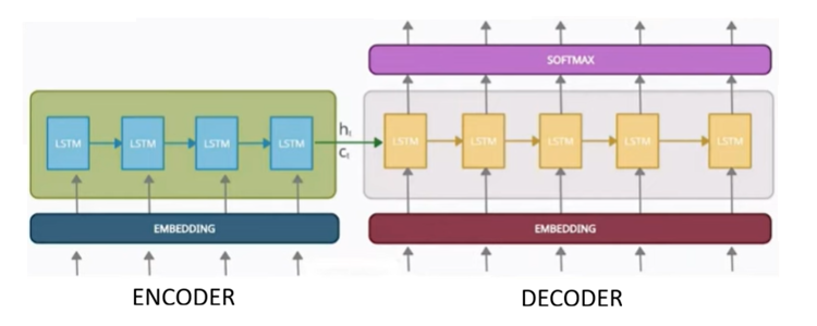
We can improve the basic encoder–decoder architecture by introducing word embeddings. Initially, words are represented using one-hot encoding. However, in real-world applications, vocabularies can contain tens or even hundreds of thousands of words. In such cases, one-hot vectors become extremely high-dimensional and inefficient.

Embeddings solve this problem by mapping words into low-dimensional dense vectors. Instead of a one-hot vector, each word is passed through an embedding layer that produces a compact numerical representation. For example, if we choose a three-dimensional embedding, each word is represented by a vector of size three.

These embeddings capture semantic information about words. Words with similar meanings tend to have similar embeddings. The embedding layer is trainable, meaning its weights are updated during training, allowing the model to learn meaningful representations of words. We can also use pre-trained embeddings such as Word2Vec or GloVe.

Embedding layers are used in both the encoder and the decoder. By doing this, the model can better capture the nuances and contextual meaning of words while keeping the input dimensionality manageable.

IMPROVEMENT 2: DEEP LSTM

Another important improvement is the use of deep LSTMs. Instead of using a single LSTM layer, we can stack multiple LSTM layers to form a deep architecture. In this setup, the input first passes through an embedding layer and then flows through multiple LSTM layers in the encoder.

Each LSTM layer processes the output of the previous layer, allowing the network to learn increasingly abstract representations. The final representations are passed to the corresponding LSTM layers in the decoder. Similarly, in the decoder, outputs from one LSTM layer are passed upward through multiple layers before reaching the final softmax layer.

Deep LSTMs help in handling long-term dependencies more effectively, especially for long sentences. They provide greater capacity to store and process information, as more parameters are available compared to a single LSTM. Another advantage is hierarchical understanding: lower layers can capture word-level patterns, middle layers can model sentence-level structure, and higher layers can capture broader contextual information.

By increasing the number of layers and parameters, the learning capacity of the model increases. This allows the model to capture subtle variations and deeper patterns in language, leading to better translation performance.

IMPROVEMENT 3: REVERSING THE INPUT

Another optimization technique is reversing the input sequence before feeding it to the encoder. In some language pairs, reversing the input helps reduce the distance between related words in the input and output sequences, making gradient propagation easier.

This technique allows the model to capture context more effectively and can improve convergence, especially for longer sentences. However, this approach does not work for all language pairs. It is mainly effective in cases where the initial words of the input sentence carry more contextual importance.

THE SUTSKEVER ARCHITECTURE

Application to Translation:

The architecture proposed by Sutskever et al. focused on translating English to French, demonstrating the effectiveness of sequence-to-sequence learning in neural machine translation.

End-of-Sentence Symbol:

Each sentence was terminated using a special end-of-sentence token <EOS>, enabling the model to recognize when to stop generating output.

Dataset:

The model was trained on a subset of 12 million sentence pairs, consisting of approximately 348 million French words and 304 million English words, collected from publicly available datasets.

Vocabulary Limitation:

To control computational complexity, fixed vocabularies were used: 160,000 most frequent words for English and 80,000 for French. Words outside these vocabularies were replaced with a special <UNK> token.

Reversing Input Sequences:

English input sentences were reversed before being fed into the encoder. This was shown to significantly improve learning efficiency, particularly for longer sentences.

Word Embeddings:

The model used 1,000-dimensional word embeddings to represent words, enabling dense and meaningful representations.

Architecture Details:

Both the encoder and decoder consisted of 4 LSTM layers, with each layer containing 1,000 units, forming a deep LSTM-based architecture.

Output Layer and Training:

A softmax layer was used to generate probability distributions over the target vocabulary. The entire model was trained end-to-end.

Performance – BLEU Score:

The model achieved a BLEU score of 34.81, outperforming the baseline statistical machine translation system, which achieved a BLEU score of 33.30. This marked a significant advancement in neural machine translation.