Gradient Boosting For Classification - 1

Now we will learn Gradient Boosting in the context of Classification

We have already learned the gradient boosting algorithm in the context of regression. The same core algorithm is also used for classification tasks — we do not need an entirely different algorithm.

The only change required is in the loss function. While regression typically uses squared error loss, classification (especially binary classification) uses the log loss (also called logistic loss or cross-entropy loss).

So, by simply replacing the loss function with one suited for classification, such as log loss, gradient boosting can be directly applied to classification problems. The rest of the algorithm — fitting regression trees to the negative gradients (pseudo-residuals), updating the model iteratively — remains exactly the same.

This flexibility is a key strength of gradient boosting: it adapts to different problem types (regression, classification, ranking) just by swapping out the loss function.

Understanding Gradient Boosting for Classification Tasks

Let’s explore how gradient boosting works in classification tasks using a small dataset. The dataset consists of 8 rows and 3 columns: cgpa, iq, and the target column is_placed (0 = Not Placed, 1 = Placed). Our goal is to predict whether a student will get placed based on their CGPA and IQ.

We will apply Gradient Boosting to this data to make predictions for new students. The idea behind gradient boosting is to build multiple weak models (typically decision trees) and combine them in a stage-wise additive manner to form a strong, ensemble model.

We define our final model as:

                                f(x) = f₀(x) + f₁(x) + f₂(x)

• f₀(x) is our initial model.

• f₁(x) and f₂(x) are models trained on the residuals or gradients of the previous model.

In regression problems, f₀(x) is usually initialized as the mean of the target values. But in classification, especially binary classification, we initialize f₀(x) using log(odds).

Step 1: Building the Initial Model f₀(x)

Since this is a classification problem, our first step is to compute the log-odds of the target classes :

In our dataset:

• Number of students placed (1s) = 5

• Number of students not placed (0s) = 3

So ,

This means that regardless of CGPA or IQ, our initial model predicts a log-odds score of 0.5108 for every student.

This value becomes our baseline prediction. The prediction table for f₀(x) will look like this :

This constant output is expected — it’s just the starting point. From here, gradient boosting proceeds to build decision trees that try to correct the error in this prediction (i.e., the residuals). These will be modeled as f₁(x), f₂(x), and so on .

Converting Log-Odds to Probability and Calculating Residuals in Classification

At this stage, we've built our initial model f₀(x) using log-odds. However, as we move forward in building the next stages of the gradient boosting model, we need to compute residuals — just like we did in regression. But here's the catch:

The quantity f₀(x) gives us log-odds, while the actual target values (like is_placed) are in probability terms (0 or 1).

We can't directly subtract log-odds from 0 or 1, because they aren't on the same scale. So, we first convert log-odds to probability.

Step 1: Convert Log-Odds to Probability

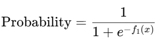
We convert log-odds to probability using the sigmoid function :

In our case, the log-odds value from the initial model f₀(x) is approximately 0.5108, so :

This means that our model is predicting a probability of 0.625 for every student, regardless of their CGPA or IQ .

Step 2: Thresholding the Prediction

Since we are dealing with a binary classification problem (Placed or Not Placed), we define a threshold (commonly 0.5) to convert the predicted probability to class labels:

• If probability ≥ 0.5 → predict 1 (Placed)

• If probability < 0.5 → predict 0 (Not Placed)

So, our initial model is blindly predicting 1 for all students. It’s not a good model — but it’s a starting point, just like using the mean in regression.

Step 3: Calculating Pseudo-Residuals

To improve the model, we now calculate residuals, which represent the mistakes made by f₀(x). Just like in regression where residuals = actual − predicted :

So we subtract the predicted probabilities from the actual outcomes :

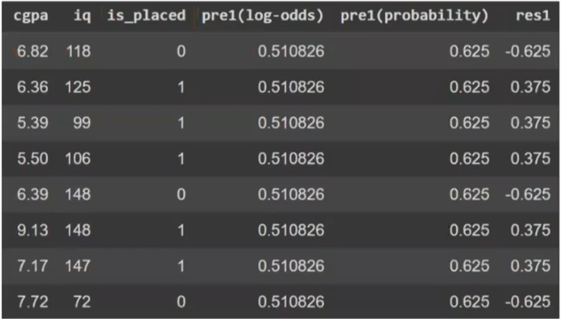
These residuals form the new target for our next model .

Step 4: Training the Next Model on Residuals

Now we train a regression decision tree (yes, regression!) using:

• Inputs: cgpa, iq

• Target/output: residuals (res1 column)

This decision tree will learn to predict the errors made by the initial model, and help us correct those errors in the next iteration.

Even though this is a classification problem, our next model is a regression tree — because we’re fitting it to numeric residuals (not class labels).

Building the Second Model: Adding a Weak Learner (Decision Tree) to Improve Predictions

In Gradient Boosting, each new model is trained to correct the errors (residuals) made by the previous model. At this point:

• We’ve trained our initial model f₀(x) using log-odds.

• We calculated residuals using the difference between true labels (is_placed) and predicted probabilities.

• Now, we train a regression tree (h₁(x)) on those residuals.

This regression tree is called a weak learner, meaning it’s a shallow decision tree — not too complex, so that it can capture basic patterns without overfitting.

Combining Models: f₁(x) = f₀(x) + h₁(x)

The next model is simply the sum of the previous prediction and the new model’s output:

                      f₁(x) = f₀(x) + h₁(x)

In regression, you can directly add the output of h₁(x) to f₀(x). But in classification, there's a subtle twist:

Our base model f₀(x) outputs log-odds, but the decision tree h₁(x) is trained on residuals (which are on the probability scale).

So we can’t directly add them — we need to convert the residuals to the log-odds space.

Formula to Convert Residuals to Log-Odds (Leaf Node Output)

To convert the residuals at each leaf node into log-odds values, we use the formula :

Where:

• Residuals are the errors from the previous model.

• p is the predicted probability from f₀(x) for each data point falling into that leaf node.

Applying the Formula to Leaf Nodes

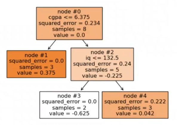
Each leaf in the tree has a set of rows (data points) that fall into it. Let’s calculate the log-odds for Node 3, where rows 1 and 8 fall:

• Residuals : -0.625, -0.625

• Probabilities : 0.625, 0.625

Now plug into the formula :

So, the output of Node 3 is −2.66 (in log-odds space).

You’ll repeat this process for all leaf nodes:

• Node 1 → 1.6

• Node 3 → -2.66

• Node 4 → 0.18

Updating Predictions Using Combined Log-Odds

Each row gets an updated prediction based on the leaf node it falls into. For example:

• Row 1 (falls in Node 3):   

  

• Row 2 (falls in Node 1):

These values are new log-odds predictions. To convert them to probabilities:

So for Row 1 :

Since this is below 0.5, we classify it as 0. That’s how gradient boosting iteratively improves predictions.

• The regression tree (h₁(x)) is trained on residuals from the initial model.

• Leaf node outputs must be converted to log-odds before being added to f₀(x).

• Updated predictions are calculated, converted to probability, and used for the next round of residuals.

• This process repeats for multiple rounds to refine predictions further.

Building the Third Model: Adding Another Tree and Controlling the Learning Rate

After combining the initial model f₀(x) with the first decision tree h₁(x), we get a new set of predictions. Based on those updated predictions, we compute a new set of residuals — let’s call them res₂ .

We then train another regression tree (h₂(x)) on these new residuals, just like we did before.

Understanding the Full Model So Far

At this point, we have built :

• One base model : f₀(x) — outputs log-odds (starting point)

• Two weak learners:

  • h₁(x) — first regression tree trained on residuals res₁

  • h₂(x) — second regression tree trained on residuals res₂

The combined model is :

This gives us predictions in log-odds form, which we then convert to probability using the sigmoid function.

Error is Decreasing Over Iterations

When we compare res₁ and res₂, we notice that residuals are getting closer to zero. This means our model is improving with each stage — it’s learning from its past mistakes.

Introducing Learning Rate (Shrinkage)

Sometimes, the updates from each tree (h₁(x), h₂(x), etc.) can be too large, causing unstable or overconfident predictions.

To control this, we introduce a learning rate (denoted as η, eta), a value between 0 and 1. It helps by shrinking the impact of each tree :

Think of the learning rate as a volume knob: it dials down how much each tree is allowed to change the model.

This is useful especially when:

• Residuals are large

• Log-odds jumps between iterations are too sharp

• Overfitting risk is high

Leaf Node Log-Odds (Decision Tree 2)

Let’s say in your second decision tree (dt2), the log-odds values in the leaf nodes are:

• Node 3: +1.09

• Node 4: −2.94

• Node 2: +1.56

You can scale these with a learning rate (e.g., η = 0.1) before adding them to the previous predictions.

Why Learning Rate Matters

• High learning rate (η → 1) → Faster training but risk of overshooting or overfitting

• Low learning rate (η → 0.1 or 0.01) → Slower training but more stable, generalizable model

A small learning rate with more trees usually gives better results. It's a tradeoff between speed and accuracy.

You’re now seeing the full power of gradient boosting:

• It builds the model in stages

• Each tree learns from the mistakes of the previous stage

• Learning rate helps control overconfidence and improve generalization

Final Model Output: Combining All Models in Gradient Boosting

At this stage, we've successfully built three models :

• The initial model f₀(x) (based on log-odds from the base rate of outcomes),

• The first decision tree h₁(x),

• The second decision tree h₂(x).

Our full ensemble model is now :

Each component contributes log-odds values, and together they give us the combined prediction in the log-odds form.

Step 1: Combine Log-Odds

We already have:

• The base model log-odds from f₀(x)

• The leaf node outputs (log-odds) from the two decision trees

For each row in the dataset, we add these three values to get the combined log-odds. This gives us a new column: pre3(log-odds).

Step 2: Convert Log-Odds to Probability

Once we have pre3(log-odds), we use the sigmoid function to convert log-odds into a probability :

This gives us pre3(probability) — the final predicted probability for each input .

Step 3: Make Predictions Using a Threshold

With predicted probabilities in hand, we use a threshold (commonly 0.5) to make a final classification:

• If pre3(probability) > 0.5, predict 1 (student is placed)

• Otherwise, predict 0 (student is not placed)

Final Table Snapshot

• We built models sequentially, each correcting the errors of the previous.

• We combined their outputs in log-odds form.

• We converted log-odds to probabilities using the sigmoid function.

• We classified the final outputs using a threshold.

That’s the magic of Gradient Boosting for Classification. It's just like regression boosting — the key difference lies in using a log loss function, working in log-odds, and converting it to probability before calculating residuals.

Prediction Using the Gradient Boosting Model

Let’s now walk through how to make a prediction for a new student using our combined gradient boosting model.

Input:

• CGPA = 7.2

• IQ = 100

Our goal: Predict whether the student will get placed or not (i.e., classify as 1 or 0).

Step-by-Step Prediction

We will use our final model :

Step 1: Base Model (f₀(x))

• This is the initial log-odds based on the entire dataset.

• From earlier, we know:

                                   f₀(x) = 0.51

Step 2: First Decision Tree (h₁(x))

• With CGPA = 7.2 and IQ = 100:

  • From the tree, this input falls into a leaf node with prediction:

                                 h₁(x) = -2.66

Step 3: Second Decision Tree (h₂(x))

• From the second tree:

  • Same input falls into the node giving output:

                                    h₂(x) = +1.56

Step 4: Final Log-Odds Calculation

Now we sum all the contributions:

Final log-odds = 0.51 + (−2.66) + 1.56 = −0.59

Step 5: Convert Log-Odds to Probability

Using the sigmoid function :

Step 6: Make Final Decision

• If probability ≥ 0.5, predict 1 (placed).

• If probability < 0.5, predict 0 (not placed).

In our case:

• Final probability = 0.35

• This is less than 0.5, so the prediction is : Not Placed

Interpretation

This is how Gradient Boosting works:

• Start simple (baseline).

• Learn from mistakes using residuals.

• Combine multiple weak learners step-by-step.

• Output final prediction in probability form.

• Use a threshold to classify.