Gradient Boosting For Regression - 2

HOW GRADIENT BOOSTING WORKS ?

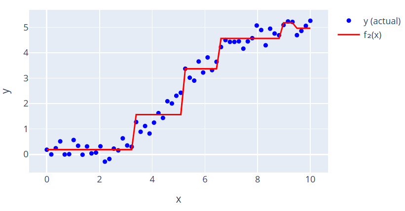
Suppose we have a dataset with one input column, "experience" (x), and one output column, "salary" (y). When we plot this data, we observe a pattern: after a certain experience level, the salary increases linearly and then becomes stagnant. Our goal is to build a model, f(x), that captures this true relationship between 'x' and 'y'.

1. Initial Model (f₀(x))

Initially, we assume no prior knowledge of the relationship. Our first model, f₀(x) , is simply the mean of the 'salary' (y) column. This means, regardless of the 'experience' value, our model always predicts the average salary.

Naturally, this initial model is not perfect and makes significant errors at many data points.

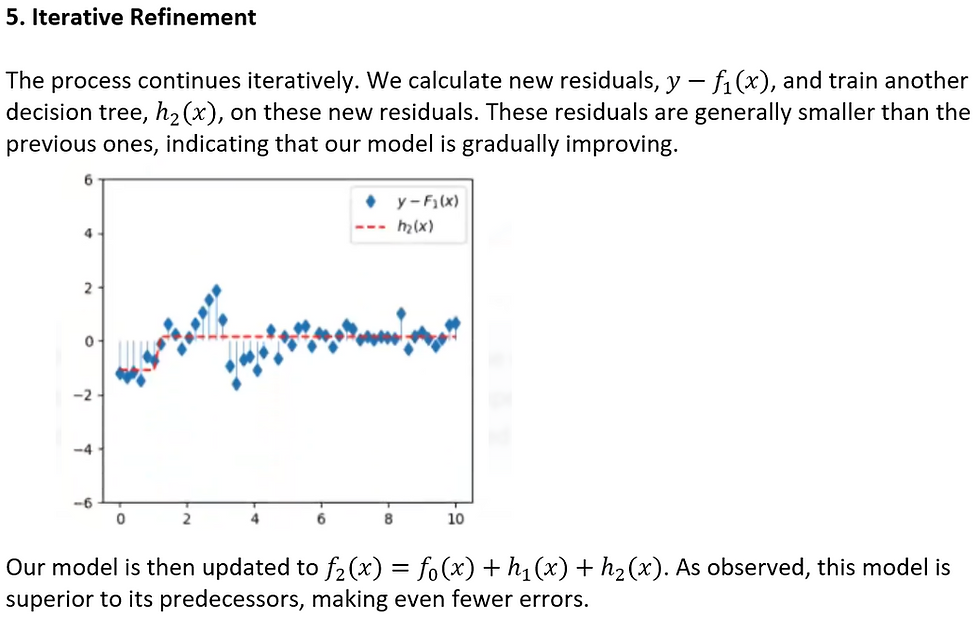
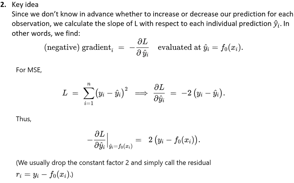
2. Calculating Residuals

Next, we calculate the residuals, which are the differences between the actual 'salary' (y)

and our model's predictions ( f₀(x) ). We then plot these residuals against the 'experience' (x) values. The scale of the y-axis (now representing residuals) changes to reflect these differences.

3. Training the First Decision Tree (h₁(x))

In gradient boosting, the crucial next step is to train a new model on these residuals. We use a decision tree, denoted as h₁(x), as our base learner. This decision tree is typically small, often containing only one node, focusing on capturing the patterns in the errors of our previous model.

We keep repeating this process. After, for example, 10 iterations, the final model, which is the sum of the initial prediction and all subsequent decision trees, effectively captures the data's pattern and significantly reduces prediction errors.

This is the core idea of how Gradient Boosting works: it sequentially builds an ensemble of weak learners (decision trees) by focusing on the errors (residuals) of the previous models, leading to a powerful predictive model.

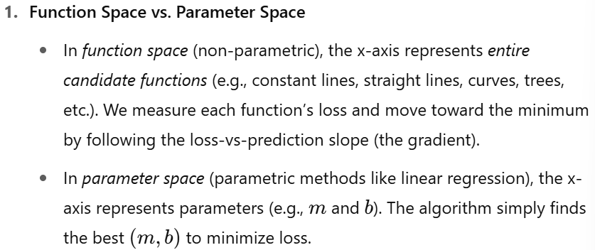
FUNCTION SPACE VS PARAMETER SPACE

We have a dataset where the x-axis represents 'experience' and the y-axis represents 'salary'. Our objective is to build a machine learning model that can predict salary based on experience. To achieve this, we've decided to apply Gradient Boosting. Our goal is to discover the underlying function, y = f(x), that describes this relationship.

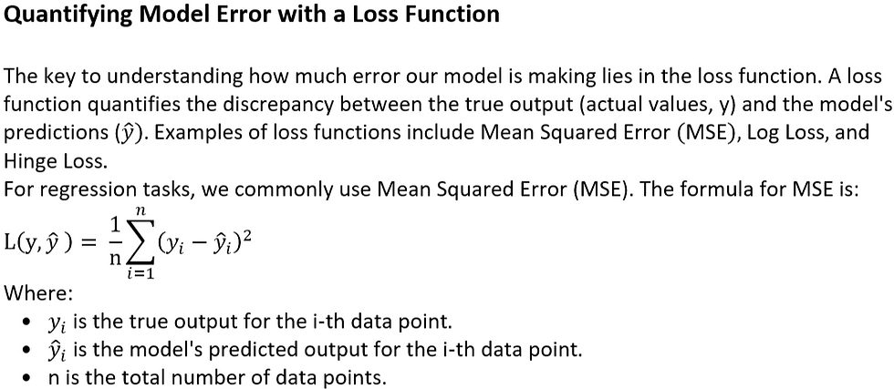
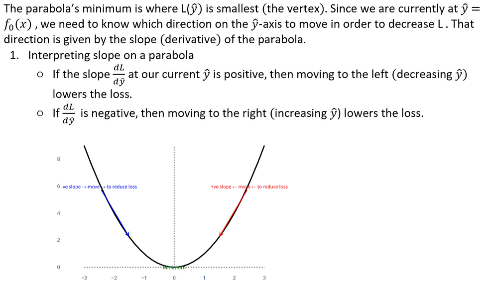
How to Reduce This Error: Understanding Function Space

The crucial question now is: how do we reduce this error ? To answer this, we need to understand the concept of function space.

Understanding Model Optimization: Functional Space vs. Parameter Space

To understand how complex algorithms like Gradient Boosting work, we need to visualize how they find the best possible model. This involves understanding the concept of a functional space.

Visualizing the Functional Space

Let's simplify the complex, multi-dimensional problem of model fitting into a 2D graph.

• The y-axis will represent the Loss (L), which tells us how bad our model's predictions are. A lower value is better.

• The x-axis will represent the different models (functions) we can use to make predictions.

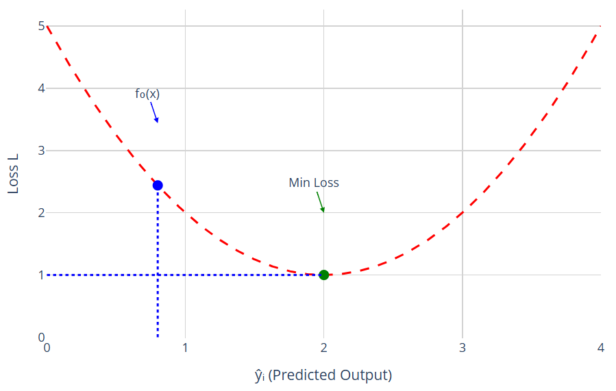
Step 1: The Initial Model

We start with a very simple, baseline model, which we'll call f₀(x). A common starting point is a model that predicts the average value of our target variable, y. Let's say the average is 20.

• Model: f₀(x) = 20

• Prediction: For every input xᵢ, the prediction ŷᵢ is 20.

• Loss: We can now calculate the total loss (e.g., using Mean Squared Error - MSE) for this model. This gives us our first point on the graph.

Step 2: Iterating and Finding Better Models

The Goal: Minimizing Loss in Functional Space

The key idea is that we can try an infinite number of functions—linear, curved, or any other mathematical form. Each function is a unique point on the x-axis of our graph. This "space" of all possible functions is called the functional space.

Our goal is to find the function f(x) that results in the minimum possible loss. This function represents the best possible model because it captures the true relationship within our data most accurately.

Contrast with Parameter Space: The Case of Linear Regression

This approach is different from simpler, parametric machine learning algorithms like Linear Regression.

A parametric algorithm assumes the form of the function from the beginning. Linear regression, for instance, assumes the relationship between the variables is always a straight line:

                              y = f(x) = mx + b

Here, the goal is not to find the type of function (it's already assumed to be linear). The goal is to find the optimal parameters (m for the slope and b for the intercept) that create the best-fitting line.

The space we search for these optimal values is called the parameter space. In this space, the axes are not functions, but the parameters themselves (m and b). For each combination of m and b, we calculate a loss. Our objective is to find the specific values of m and b that correspond to the lowest point on the loss curve.

Function Space vs Parameter Space

• In parametric algorithms (e.g., Linear Regression), the model assumes a specific function form :

                             y = f(x) = mx + b

  • The algorithm doesn’t find the function form—it only finds the best parameters m and b

  • So the graph has parameters on x-axis → it's called parameter space

• In non-parametric algorithms (e.g., Gradient Boosting):

  • We don’t assume the function form in advance

  • We try many possible functions (additive models, trees, etc.)

  • So the x - axis holds entire functions → it's called function space

Summary of Key Differences

Feature	Functional Space (e.g., Gradient Boosting)	Parameter Space (e.g., Linear Regression)
What's on the x-axis?	Entire functions: f₀(x) , f₁(x) etc.	Model parameters: m, b, etc.
What is the goal?	To find the optimal function that minimizes loss.	To find the optimal parameters for a pre-defined function.
Model Type	Typically non-parametric. It does not assume the data follows a specific structure.	Parametric. It assumes the data follows a specific structure (e.g., a line).

DIRECTION OF LOSS MINIMIZATION

1. Our Dataset and Initial Scatter Plot

4. How Do We Move Toward Minimum Loss ?

5. Computing Residuals for Each Data Point

6. Fitting the First Decision Tree to Residuals

7. Updating the Model and Proceeding to f₁(x)

8. Recap of Key Concepts

Update the Function in Gradient Boosting

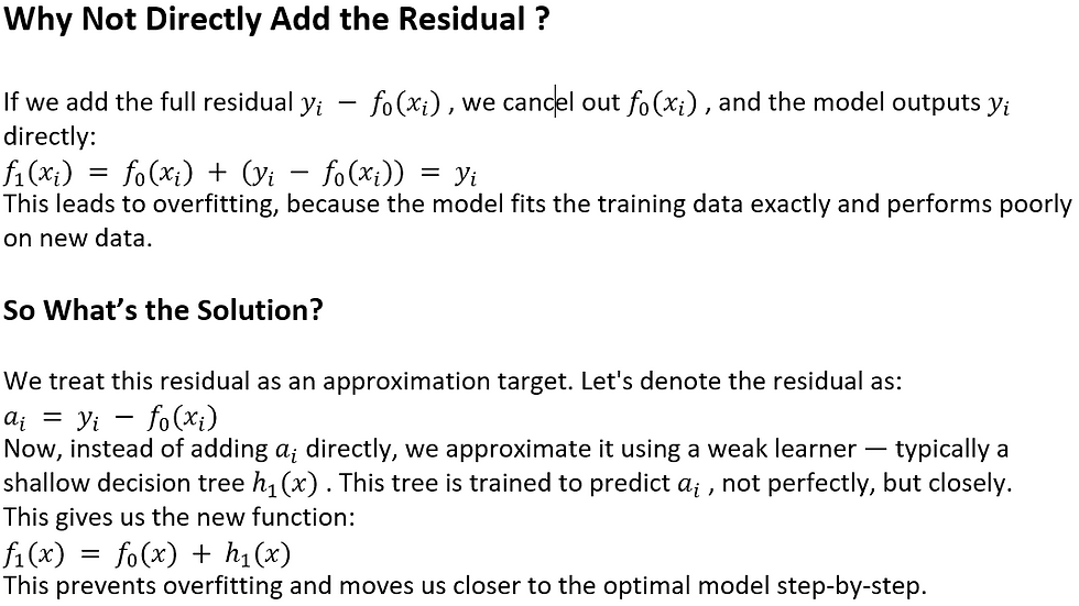
Moving in Function Space

As we continue training our model using weak learners, we are not just updating predictions — we are navigating the loss surface in function space.

Each weak learner points in the direction of steepest descent, and we take a step along that direction to reduce the loss.

You can imagine this process like moving on a 2D terrain where the height represents loss (error), and each move with a weak learner is a small step downhill toward the minimum.

• We start at an initial point F₀(x) (e.g., mean).

• Each weak learner (like h₁, h₂, ...) pushes us a little closer to the best possible model.

• After n steps, Fₙ(x) becomes a good approximation of the true function.

The figure below shows how each updated model moves us closer to the optimal prediction (minimum loss):

What This Shows:

• A contour plot of a convex loss surface (like MSE).

• Each F₀, F₁, F₂ ... point is a stage in boosting.

• The steps visually represent how gradient boosting minimizes loss by moving in the direction of the negative gradient in function space.

Final Summary

• At each step, we:

  1. Compute the residual.

  2. Train a weak learner to predict it.

  3. Add the weak learner to the previous model.

• This gradually builds a strong predictive model.

• It avoids overfitting by using weak learners and only partially correcting errors.

Intuition Behind Gradient Boosting (Golf Player Analogy)

Imagine a golf player aiming to putt a ball into a hole—the hole represents the true value y, and the player's goal is to reach it with a series of shots.

Iterative Process in Gradient Boosting

Gradient Boosting builds the model step-by-step. Let’s walk through the process using the following steps :

Final Outcome

ANOTHER PERSPECTIVE OF GRADIENT BOOSTING

Let’s understand Gradient Boosting from a more intuitive, visual perspective using the golfer analogy.

Imagine a golfer (our model) trying to reach a target flag (the correct prediction y) on a loss landscape (such as the MSE loss function curve).

Conceptual Insight

This is very similar to gradient descent, but with a key difference:

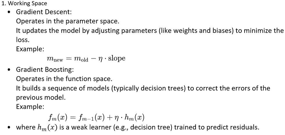
• Gradient Descent:

  Moves in parameter space by updating weights using gradients.

• Gradient Boosting:

  Moves in function space by sequentially adding weak learners that correct the residuals (gradient of loss) from the previous model.

Summary

What gradient descent does in parameter space, gradient boosting does in function space. Each step is like a controlled shot in the right direction using weak learners to gradually reach the goal.

Difference Between Gradient Descent and Gradient Boosting

Gradient Descent and Gradient Boosting are both optimization strategies, but they work in different spaces and follow different update rules.

Advantages of Gradient Boosting

Gradient Boosting is one of the most powerful machine learning techniques. Below are its key advantages:

1. High Predictive Accuracy

• Gradient Boosting often delivers state-of-the-art performance in both regression and classification tasks.

• It minimizes errors stage-by-stage, which leads to highly accurate models.

2. Handles Non-Linear Data Well

• Since it builds an ensemble of decision trees, it can capture complex, non-linear relationships in the data.

3. Feature Importance

• It naturally provides feature importance scores, helping you understand which features are most influential.

4. Robust to Overfitting (with Regularization)

• Techniques like:

  • shrinkage (learning rate),

  • limiting tree depth,

  • subsampling

    help reduce overfitting, making it more generalizable than simple ensembles.

5. Flexible Framework

• It can optimize different loss functions (e.g., MSE, MAE, log-loss).

• It can also be adapted to ranking, classification, and other tasks.

6. Works with Missing Data

• Some implementations like XGBoost and LightGBM can handle missing values internally.

 7. No Need for Feature Scaling

• Unlike models like SVM or Logistic Regression, Gradient Boosting doesn’t require normalization or standardization of features.

 8. Custom Loss Functions

• You can define and plug in custom loss functions depending on the problem, which gives high flexibility.