Gradient Descent

Understanding Gradient Descent : The Foundation

Gradient Descent is a fundamental, first-order iterative optimization algorithm widely used in machine learning and deep learning. Its primary goal is to find a local minimum of a differentiable function. Think of it like a hiker trying to find the lowest point in a valley while blindfolded. Since they can't see the entire landscape, they rely on the slope of the ground directly beneath their feet to decide which way to move.

The Core Idea: Following the Steepest Descent

The central idea behind Gradient Descent is to take repeated steps in the opposite direction of the gradient of the function at the current point. Why the opposite direction? Because the gradient itself points in the direction of the steepest ascent – the direction where the function's value increases most rapidly. Therefore, to minimize the function, we must move in the exact opposite direction, which corresponds to the steepest descent. Each step aims to move us closer to a lower point in the function's landscape.

In practical applications, especially with complex functions or large datasets, we might sometimes use an approximate gradient, but the principle remains the same: we're always trying to move "downhill."

Gradient Ascent: The Opposite Approach

Conversely, if we were to take steps in the direction of the gradient, the procedure would be known as Gradient Ascent. As you might infer, Gradient Ascent is used to find a local maximum of a differentiable function. It's the inverse operation, seeking the "peak" instead of the "valley."

Applying Gradient Descent to Linear Regression

Let's consider a scenario where we have a dataset with 4 rows and 2 columns, representing cgpa and placement records for 4 students. Our objective is to find the best-fit line that describes the relationship between cgpa (input feature, xᵢ ) and placement (output, yᵢ ). This involves finding the optimal values for the slope (m) and the y-intercept (b) of the line y = mx+b, such that the error is minimized.

The Loss Function: Quantifying Error

To quantify the "error" of our line, we use a Loss Function (also known as a Cost Function). For linear regression, a common choice is the Mean Squared Error (MSE), or in this case, the Sum of Squared Errors :

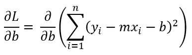
Here, yᵢ​ is the actual placement value for the i-th student, and ŷᵢ ​is the predicted placement value from our line. Since ŷᵢ = mxᵢ+b , the loss function can be written as :

This function is dependent on the values of m and b. As we change m and b, the value of the loss function, L(m,b), will also change. Our goal is to find the m and b values that yield the minimum possible L(m,b).

Simplifying the Problem: Optimizing for 'b'

For simplicity, let's assume we already know the optimal value of m, say m = 78.35. In this case, our loss function becomes a function solely of b :

When L(b) is plotted against b, it forms a parabolic graph (a U-shaped curve). Our task now is to find the value of bat the bottom of this parabola, where L(b) is at its minimum. This is where Gradient Descent comes into play.

Steps for Gradient Descent (Optimizing 'b'):

To find the minimum value of busing Gradient Descent, we follow these iterative steps:

1. Initialize b(Random Start):

• We start by picking a random initial value for b. Let's say, we select b_old ​= −10. This is our starting point on the parabolic curve.

2. Calculate the Slope (Gradient) at the Current Point:

• To know which way to move downhill, we need to determine the slope (gradient) of the loss function L(b) at our current b_old ​value. This is done by taking the derivative of L(b) with respect to b, and then plugging in the current b_old ​value.

• The derivative ∂L/∂b ​tells us the direction and steepness of the slope.

3. Update b (Moving Downhill) :

• The core idea of Gradient Descent is to move in the opposite direction of the gradient.

• If the slope is negative (meaning we are on the left side of the minimum), we need to increase b to move towards the minimum.

• If the slope is positive (meaning we are on the right side of the minimum), we need to decrease b to move towards the minimum.

• Initially, the update rule might seem like: b_new = b_old - slope

• Example without Learning Rate:

  • If the slope is −50(meaning a steep downhill on the left): b_new ​= −10−(−50) = 40.

  • If the slope is 50(meaning a steep uphill on the right): b_new​ = −10−(50) = −60.

• Problem : As seen in the example, a direct subtraction of the slope can lead to drastic changes in b, potentially causing "zig-zag" movements and overshooting the minimum. The algorithm might even diverge instead of converging.

4. Introducing the Learning Rate (η): Controlled Steps:

• To prevent drastic changes and ensure controlled convergence, we introduce a crucial hyperparameter called the learning rate (η). The learning rate scales the step size, ensuring we take smaller, more precise steps.

• The refined update rule becomes:

  b_new = b_old - η . slope

• Example with Learning Rate: Let's set η = 0.01

  • If the slope is −50 :

    b_new ​= −10−(0.01 ⋅ −50) = −10−(−0.5) = −10+0.5 = −9.5

  • If the slope is 50 :

  ​ b_new= −10−(0.01 ⋅ 50) = −10−0.5 = −10.5

• Notice how the learning rate helps us take smaller, more manageable steps, preventing us from overshooting. We repeat this process:

calculate the new slope at b_new ​, and update b again using the learning rate.

When to Stop ? (Convergence Criteria)

The iterative process of updating b continues until we reach a point where further updates yield negligible changes, indicating that we are very close to the minimum. We can define stopping criteria based on:

1. Small Change in b :

   Stop when the absolute difference between b_new ​and b_old​ is very small, e.g., ∣b_new ​− b_old ​ ∣ ≤ 0.0001. This suggests that the updates are becoming minuscule, meaning we're near a flat part of the curve (the minimum).

   
   

2. Maximum Number of Iterations (Epochs):

   Set a predefined maximum number of iterations (epochs), e.g., 1000 or 100. This acts as a safeguard to prevent the algorithm from running indefinitely, especially if it struggles to converge or the loss function has a very flat minimum.

By carefully applying these steps and criteria, Gradient Descent efficiently navigates the loss landscape to find the optimal parameters that minimize the error.

Mathematical Intuition Behind Gradient Descent

As established, our goal is to find the best-fit line by minimizing the loss function L(m,b). For this specific example, we're assuming m = 78.35 is known, and we only need to find the optimal value for b.

The Iterative Update Process

Gradient Descent works iteratively. We start with a random initial guess for band then repeatedly update it in the direction that reduces the loss.

Initialize b and Set Up the Loop

• We begin by choosing an arbitrary initial value for b, say b_old ​. This value can be anything.

• The core of Gradient Descent is an iterative loop that runs for a predetermined number of epochs (iterations) or until a convergence criterion is met.

  For each epoch, the update rule for b is:

  b_new = b_old - η⋅slope

  Here, η is the learning rate, a small positive value (e.g., 0.01) that controls the step size.

Calculating the Slope (Gradient)

To calculate b_new ​, we first need to determine the slope of the loss function with respect to bat our current b_old ​value. This "slope" is precisely the partial derivative of the loss function L with respect to b, denoted as ∂L/∂b .

Our loss function is :

 Substituting ŷᵢ = mxᵢ+b :

Now, let's differentiate L with respect to busing the chain rule :

We can pull the summation sign out :

Applying the chain rule, where u = (yᵢ - mxᵢ - b) and ∂u/∂b = -1 :

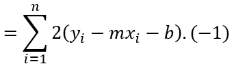
So, the slope (gradient) of the loss function with respect to b is :

Example Calculation

Let's assume, for a specific iteration, we want to calculate the slope when b = 0 and m = 78.35.

Substituting these values into the slope formula:

By plugging in the actual data values for xᵢ ​and yᵢ ​from our dataset into this formula, we would obtain a numerical value for the slope at b = 0.

The Iterative Update in Action

Once we have calculated the slope for the current b_old ​(e.g., at b = 0), we can then compute the b_new value using our update rule. For instance, if η = 0.01 :

b_new = b_old - (0.01 * slope)

This process is then repeated for a specified number of epochs. In each epoch:

1. We calculate the slope of the loss function at the current b_old ​.

2. We update b_old ​to b_new ​using the learning rate and the calculated slope.

3. The new b_new ​becomes the b_old​ for the next iteration.

By repeatedly taking these small steps in the direction opposite to the gradient, we gradually descend the loss landscape, ultimately converging towards the value of b that minimizes the loss function.

Generalizability of the Formula

The fundamental update formula, b_new ​= b_old ​− η⋅slope , is highly versatile and not limited to just linear regression. Its power lies in its generality :

• For any machine learning algorithm, as long as you can define a differentiable loss function and calculate its partial derivative (gradient) with respect to the parameters you want to optimize, you can use a similar Gradient Descent update rule.

• By simply changing the loss function and its derivative, this same principle allows us to find the optimal values for various parameters in different machine learning algorithms (e.g., weights in neural networks, parameters in logistic regression, etc.).

This mathematical intuition forms the backbone of how many modern machine learning models learn from data.

Effect of Learning Rate (η)

The learning rate (η) is a crucial hyperparameter in Gradient Descent that dictates the size of the steps taken towards the minimum of the loss function. Its value significantly influences the training process and the algorithm's ability to converge.

• Learning Rate is Too Small (Underfitting): If η is set to a very small value, the algorithm will take tiny steps. While it may eventually reach the minimum, it will do so very slowly, requiring a large number of epochs. This can lead to excessively long training times.

• Learning Rate is Optimal: An optimal learning rate allows the algorithm to converge efficiently. It takes steps large enough to make good progress each epoch but small enough to avoid overshooting the minimum. This leads to convergence in a reasonable number of epochs.

• Learning Rate is Too High (Overshooting/Divergence): If ηis too large, the algorithm might take steps that are too big, causing it to overshoot the minimum repeatedly. Instead of converging, the loss might fluctuate wildly, increase, or even diverge, meaning it never reaches the minimum loss and fails to learn effectively.

Effect of Loss Function Landscape

The shape of the loss function itself plays a critical role in how Gradient Descent performs.

• Convex Functions (Ideal Scenario):

  • A convex loss function has a single, bowl-shaped curve with only one global minimum. This is the ideal scenario for Gradient Descent because it guarantees that the algorithm, if properly configured, will always converge to this unique global minimum, regardless of the starting point.

• Non-Convex Functions (Challenges):

  • Non-convex loss functions are common in more complex models (like deep neural networks). They can have multiple local minima in addition to a global minimum.

    • Local Minima: If Gradient Descent starts in a region closer to a local minimum, it might get "stuck" there, failing to reach the true global minimum. This means the algorithm might settle for a "good enough" solution rather than the best possible one.

    • Saddle Points: These are points where the slope is zero (like a minimum in one direction and a maximum in another), but they are not true minima. Gradient Descent can get very slow around saddle points, as the gradient becomes very small, making it difficult to escape. Flat Surfaces or Plateaus: Regions with very small gradients (flat surfaces or plateaus) can also slow down Gradient Descent significantly. The algorithm makes tiny updates, taking a very long time to traverse these areas. If the number of epochs is set too low, the algorithm might stop prematurely before it has had a chance to move past these flat regions and reach a deeper minimum.

Understanding both the learning rate's influence and the geometry of the loss function is crucial for effectively training machine learning models with Gradient Descent.

Local Minima and Saddle Points in Gradient Descent

When training machine learning models, Gradient Descent (GD) is the most common optimization algorithm used to find the best set of parameters that minimize a loss function. We can imagine this loss function as a multi-dimensional landscape, where the "height" represents the loss and the "horizontal dimensions" represent the model's parameters. The goal of GD is to descend this landscape to find the lowest point.

Global Minimum

The global minimum is the point in the loss landscape where the loss function reaches its absolute lowest value. It represents the optimal set of parameters that make the model perform the best. In an ideal scenario, gradient descent aims to converge to this point.

Local Minima

A local minimum is a point where the loss function's value is lower than at all neighboring points, but it's not the absolute lowest value across the entire landscape. Imagine small dips or valleys on a mountain range, where each dip is lower than its immediate surroundings, but the actual lowest point (global minimum) might be much further away.

• Challenge for GD: If gradient descent starts in a region whose path leads to a local minimum, it might get "stuck" there. Since the gradient at a local minimum is zero (or very close to zero), the algorithm believes it has found the lowest point and stops updating, even if a better, global minimum exists elsewhere.

• Visual Cue: In the figure, you might see some paths converging to a higher "dip" on the surface, indicating a local minimum rather than the very bottom.

Saddle Points

A saddle point is a critical point where the gradient of the function is zero, similar to a minimum or maximum, but it's neither. At a saddle point, the function curves upwards in some directions and downwards in others. Think of a riding saddle: it's a minimum along one axis (from front to back) but a maximum along another (from side to side).

• Challenge for GD: Gradient descent can slow down drastically or even get "stuck" at saddle points. While the gradient is zero, it's not a minimum, and the algorithm needs a "kick" to move away from it. In high-dimensional spaces, saddle points are far more common than local minima.

• Visual Cue: In the figure, a path might flatten out or oscillate in a specific region without reaching a deep minimum, potentially indicating it's near or traversing a saddle point.

Why These Are Challenges for Gradient Descent

The existence of local minima and saddle points, particularly in the complex, non-convex loss landscapes of deep neural networks, poses significant challenges for optimization:

1. Suboptimal Solutions: Gradient descent might converge to a local minimum instead of the global minimum, leading to a model that performs worse than it could.

2. Slow Convergence: Getting stuck at or slowly moving through saddle points can drastically increase the training time.

3. Sensitivity to Initialization: As shown in the visualization, the starting point plays a crucial role. Different initial parameters can lead the algorithm to different minima.

Visual Interpretation from the Figure

In the provided 3D visualization:

• The colored surface represents the non-convex loss function, showcasing its various dips (minima) and flatter regions (potentially saddle points).

• Each distinct colored path illustrates a separate run of gradient descent starting from a different initial position.

• Observe how some paths might lead to deeper parts of the landscape (closer to the global minimum), while others might settle in shallower depressions (local minima).

• If any path seems to linger or oscillate in a flatter region without clear progress downwards, that could be an indication of it being influenced by a saddle point.

Mitigation Strategies

To overcome these challenges, various techniques are employed:

• Stochasticity: Methods like Stochastic Gradient Descent (SGD) and Mini-Batch Gradient Descent introduce randomness (noise) into the gradient calculation. This "noise" can help the optimizer "jump out" of local minima or navigate saddle points.

• Momentum: Techniques like Momentum, Adam, or RMSprop help accelerate gradient descent, particularly through flat regions or saddle points, by incorporating a fraction of the previous update into the current one.

• Adaptive Learning Rates: Optimizers like Adam, RMSprop, and Adagrad dynamically adjust the learning rate for each parameter, allowing them to take larger steps in flatter regions and smaller steps in steeper ones, which can help in navigating complex landscapes.

Batch Gradient Descent for Multiple Linear Regression

We are now extending Gradient Descent to multiple linear regression, where the output variable depends on multiple input features. Consider a dataset with three columns: cgpa (x₁​), iq (x₂), and lpa (y). We aim to model the relationship as:

ŷ = β₀ + β₁x₁ + β₂x₂

Here, ŷ ​is the predicted lpa, β₀ ​is the intercept, and β₁,β₂ ​are the coefficients for cgpa and iq respectively. Our objective is to find the optimal values for (β₀,β₁,β₂) that minimize the prediction error.

1. Initialization of Parameters

As a common practice, we initialize the parameters with some starting values.

• The intercept β₀ ​is typically set to 0.

• Other coefficients (β₁,β₂) are often initialized to 1.

So, our initial parameters are β₀ ​= 0, β₁ = 1, and β₂ ​= 1.

2. Hyperparameter Selection

Before starting the iterative process, we define the hyperparameters:

• Epochs: The total number of iterations for the algorithm (e.g., epochs = 100).

• Learning Rate (η): The step size for each update (e.g., η = 0.1).

3. The Iterative Update Process

In each epoch, we will update each parameter (β₀,β₁,β₂​) using the Gradient Descent rule:

This means we need to calculate the partial derivative of the loss function with respect to each β parameter.

The Loss Function

For multiple linear regression, we typically use the Mean Squared Error (MSE) as the loss function. When considering the entire dataset for each update, it's called Batch Gradient Descent.

This loss function for three variables (β₀,β₁,β₂​) can be visualized as a 4D graph (with the fourth dimension representing the loss value). Our goal is to navigate this 4D space to find the minimum loss.

Let's consider your example data (n = 2) :

For n = 2 data points, the expanded loss function is :

Calculating the Gradients (Partial Derivatives)

Now, we compute the partial derivatives of the loss function with respect to each parameter.

1. Gradient with respect to β₀​ (​​∂L/∂β₀ ​) :

This derivative represents the average of the negative errors.

2. Gradient with respect to β₁​ (​​∂L/∂β₁ ​) :

3. Gradient with respect to β₂​ (​∂L/∂β₂ ​):

   
   

Similarly, for β₂​ ​:

Generalizing the Gradient Calculation

For any coefficient βⱼ ​(where j > 0 corresponds to a feature xⱼ​) :

These generalized formulas allow us to calculate the slope for each parameter using the entire dataset (hence "Batch" Gradient Descent) in every iteration. The parameters are then updated simultaneously using these calculated gradients and the learning rate, driving them towards the values that minimize the overall loss.

Types of Gradient Descent

(i) Batch Gradient Descent (BGD)

Batch Gradient Descent (BGD) is the general or standard form of the Gradient Descent algorithm. In this approach, to find the error and update the model's parameters, we evaluate all training examples in the dataset. This comprehensive evaluation results in a single, precise gradient calculation, which is then used to update the model parameters. This entire procedure—processing all training examples and performing one parameter update—constitutes a single training epoch.

In simpler terms, BGD is a "greedy" approach because it considers the complete picture (all data points) to determine the best direction for parameter updates in each step. This involves summing up the errors and gradients across all examples before making any adjustment.

Advantages of Batch Gradient Descent:

• Less Noisy Updates: Since the gradient is computed over the entire dataset, it provides a very accurate and less noisy estimate of the true gradient of the loss function. This makes the optimization path smoother compared to other variants.

• Stable Convergence: BGD typically leads to stable gradient descent convergence. Because each step is based on the true gradient, it directly moves towards the minimum of a convex function, ensuring a consistent reduction in loss.

• Computational Efficiency (Resource Utilization): While it can be slow for large datasets, it is computationally efficient in terms of utilizing available resources. As all training samples are processed together, it can leverage vectorized operations, which are often optimized for parallel computation.

(ii) Stochastic Gradient Descent (SGD)

Stochastic Gradient Descent (SGD) is a variant of Gradient Descent that operates differently from its batch counterpart. Instead of processing the entire dataset at once, SGD runs one training example per iteration. In other words, for each individual training example within a dataset, SGD computes the gradient and updates the model's parameters immediately. This means that if you have 1000 training examples, SGD will perform 1000 parameter updates within a single epoch.

Since SGD processes only one training example at a time, it requires significantly less memory allocation compared to Batch Gradient Descent, making it easier to store in allocated memory, especially for very large datasets.

However, this rapid, per-example update comes with trade-offs:

• Computational Efficiency Losses (Frequent Updates): While it processes individual examples quickly, the frequent updates (one for each example) can lead to computational overhead. Each update might not be as "smooth" or precisely directed as in BGD, potentially requiring more overall iterations to converge and losing some computational speed that comes from vectorized operations in batch processing.

• Noisy Gradient: Due to these frequent updates based on just one example's gradient, the path taken by SGD towards the minimum is often much noisier and more erratic than that of BGD. The gradient estimate at any given step is less accurate because it doesn't represent the overall trend of the entire dataset.

Despite the noise, SGD's characteristics can sometimes be advantageous:

• Escaping Local Minima: The inherent "noise" can be a blessing in disguise, particularly in non-convex loss landscapes (common in deep learning). The erratic updates might allow SGD to escape shallow local minima and potentially find a better (or even global) minimum that BGD might get stuck in.

• Finding Global Minimum (Potential): While not guaranteed, the ability to jump out of local minima increases the chances of ultimately converging closer to the global minimum, especially in complex landscapes.

Advantages of Stochastic Gradient Descent:

• Memory Efficiency: It is easier to allocate in desired memory because it processes only one training example at a time, making it suitable for training with large datasets that might not fit into memory.

• Faster Computation per Update & for Large Datasets: Although it has noisy updates, each individual update is relatively fast to compute as it involves only one example. More importantly, for very large datasets, SGD can be more efficient and faster to converge than Batch Gradient Descent in terms of wall-clock time, as it starts making progress and updating parameters much more frequently than BGD (which waits for the entire dataset).

(iii) Mini-Batch Gradient Descent (MBGD)

Mini-Batch Gradient Descent (MBGD) strikes a balance between the extremes of Batch Gradient Descent (BGD) and Stochastic Gradient Descent (SGD). It is, as the name suggests, a combination of both.

Instead of using the entire dataset (like BGD) or a single example (like SGD) for each update, MBGD divides the training dataset into small, fixed-size batches (also known as "mini-batches"). The model parameters are then updated using the gradient calculated from each mini-batch separately.

For example, if you have 1000 training examples and a mini-batch size of 100, then within one epoch, MBGD will perform 10 parameter updates (1000 examples / 100 examples per batch = 10 batches).

This approach offers a pragmatic solution that leverages the advantages of both BGD and SGD:

• Balanced Computational Efficiency: By splitting the training dataset into smaller batches, MBGD maintains much of the computational efficiency gained from vectorized operations in BGD, without requiring the entire dataset to fit into memory at once. It processes multiple examples per update, which is faster than SGD's single-example processing.

• Reduced Gradient Noise: The gradient calculated from a mini-batch is a more representative estimate than a single-example gradient in SGD, leading to less noisy gradient updates compared to SGD. This results in a smoother and more stable convergence path than SGD.

• Faster Convergence & Escape Local Minima (compared to BGD): While less noisy than SGD, the inherent variability introduced by using mini-batches (rather than the full batch) can still help MBGD escape shallow local minima in non-convex landscapes, similar to SGD. Moreover, it often converges faster than BGD because it performs more updates per epoch.

Mini-Batch Gradient Descent is the most commonly used variant of Gradient Descent in deep learning and other machine learning applications today, precisely because it offers this optimal balance of training speed, stability, and memory efficiency.

Interpretation of the Figure : Trajectories of Gradient Descent Variants

The plot above visualizes how three popular variants of gradient descent — Batch, Stochastic, and Mini-Batch — update their parameters (w) across training epochs, as they attempt to converge toward the optimal solution (at w = 3).

Batch Gradient Descent (Yellow Solid Line with Circles)

• Path: Smooth, controlled, and gradually converging to the minimum.

• Behavior: It uses all training samples to compute the gradient at each step. This makes the path stable and noise-free, but also computationally heavier and slower in real-world, large-scale scenarios.

• Ideal Use Case: When training time isn't a constraint and precision is a priority — like on small datasets or in analytical experiments.

 Stochastic Gradient Descent (Orange Dashed Line)

• Path: Shaky and erratic, with visible jitters and fluctuations.

• Behavior: Makes updates using only one randomly selected sample per step. This leads to frequent oscillations, but each update is very fast.

• Benefit: It may bounce out of local minima and reach a better global solution in some non-convex loss functions.

• Trade-off: Less stable convergence. It reaches near the optimal point but doesn’t settle cleanly.

 Mini-Batch Gradient Descent (Red Dash-Dot Line with Squares)

• Path: Smooth like Batch, but quicker and more adaptable — best of both worlds.

• Behavior: Uses small random subsets (mini-batches) of the dataset (e.g., 32, 64 samples). This adds some controlled noise, helping it converge faster than Batch but more reliably than SGD.

• Sweet Spot: This is the standard in deep learning, offering high performance with good stability.

• Observation: In the figure, Mini-Batch quickly approaches w = 3 and remains tightly clustered around it, outperforming SGD in terms of stability.

Final Notes

• All three methods aim to find the same goal: the optimal parameter value w = 3.

• Batch takes the most accurate route but with higher cost.

• SGD is fast and noisy, like trial and error on steroids.

• Mini-Batch offers a practical balance — it’s what you actually use in real models.