Support Vector Machine (SVM) – Part 2

Problems with Hard Margin SVM

The hard margin Support Vector Machine (SVM) is designed under the assumption that the data are perfectly linearly separable. While this model performs well when this condition holds, it becomes inapplicable if even slight violations occur. In real-world datasets, perfect linear separability is rare due to noise, outliers, and inherent overlaps between classes. Consequently, the hard margin SVM is not practically suitable for most real-world applications.

Formally, the objective of hard margin SVM is to maximize the margin between the two classes. The optimization problem is given by :

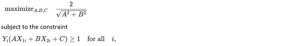
where A, B, and C are the coefficients defining the decision boundary, X¹ⁱ and X²ⁱ are the feature values for the iᵗʰ sample, and Yᵢ ∈ {+1, -1} represents the corresponding class label.

Here, the constraint Yᵢ(AX₁ᵢ + B X₂ᵢ + C) ≥ 1 enforces that all positive samples must lie on one side of the margin, and all negative samples on the other side, without any violations. Specifically :

The critical limitation arises from the strictness of these constraints. If any data point does not satisfy the margin condition, no solution exists under the hard margin SVM formulation. For example, if a red point appears in the region where green points are expected (or vice versa), the model becomes infeasible. In realistic datasets, where overlaps and noise are common, such strict separation is unattainable, rendering hard margin SVM practically ineffective.

To overcome this, the concept of slack variables is introduced. Slack variables (ξᵢ) allow controlled violations of the margin constraint, relaxing the conditions to :

This relaxation permits some points to lie inside the margin or even on the wrong side of the decision boundary, at a penalized cost. The resulting method is known as soft margin SVM, which balances maximizing the margin and minimizing classification errors.

Thus, the inflexibility of the hard margin SVM leads directly to the development of the soft margin SVM, providing the robustness needed to handle real-world, non-linearly separable data.

Slack Variables

The concept of slack variables was introduced by Vladimir Vapnik in 1995 to extend the applicability of Support Vector Machines (SVMs) to datasets that are not perfectly linearly separable. In such cases, the soft-margin SVM formulation is used, which allows for some degree of classification error by introducing flexibility into the margin constraints.

Mathematically, for each data point i, a slack variable ξᵢ ≥ 0 is introduced. The slack variable ξᵢ quantifies the degree of violation of the margin constraint for the data point xᵢ .

The interpretation of the slack variable ξᵢ is as follows :

• ξᵢ = 0 if xᵢ lies on the correct side of the margin (i.e., correctly classified with sufficient margin).

• 0 < ξᵢ ≤ 1 if xᵢ is correctly classified but lies within the margin (i.e., on the correct side of the hyperplane, but too close to it).

• ξᵢ > 1 if xᵢ is misclassified (i.e., on the wrong side of the hyperplane).

Support Vector Machines (SVM) : Slack Variables and Hinge Loss

Support Vector Machines aim to find the optimal separating hyperplane that maximizes the margin between two classes. However, when the data is not linearly separable, we introduce slack variables ξᵢ to allow certain margin violations.

Slack Variable ξᵢ : Definition

For a dataset with n samples, we compute a slack variable ξᵢ for each sample i, such that :

These variables measure how much a data point violates the margin or the classification boundary.

Case 1 : Perfect Classification

Suppose the data points are such that each one lies on the correct side of the margin :

• All positive class points lie above the positive margin.

• All negative class points lie below the negative margin.

• No points violate the margin or cross the decision boundary.

Then for all i :

                            ξᵢ = 0

This means the classifier has perfectly separated the data without any margin violations or misclassifications.

Case 2 : Margin Violation and Misclassification

Now, consider a scenario where some points do not lie strictly outside the margins.

Correctly Classified but Inside Margin :

• A positive class point lying between the hyperplane and the positive margin, or

• A negative class point lying between the hyperplane and the negative margin :

                                              0 < ξᵢ < 1

This indicates a margin violation without misclassification.

Misclassified Points :

• A positive class point lying below the hyperplane, or

• A negative class point lying above the hyperplane :

                                                    ξᵢ ≥ 1

These are misclassified points with higher slack values.

Connection to Hinge Loss and Optimization

• The slack variable ξᵢ corresponds directly to the hinge loss in SVM.

• In the SVM primal optimization problem, we minimize both the margin width and the total hinge loss :

Here, C is a regularization parameter controlling the trade-off between margin maximization and classification error.

Important Note :

In learning contexts, slack variable and hinge loss refer to the same underlying value.

You may also hear ξᵢ called the misclassification score in some explanations.

Understanding Slack Variables ( ξᵢ ) and Hinge Loss in SVM

To quantify margin violations or misclassifications, SVM introduces the hinge loss function (or slack variables ξᵢ). This helps in optimizing classification when data points are not linearly separable.

Hinge Loss Formula

For a given data point (xᵢ , yᵢ), where yᵢ ∈ {−1 , +1}, the hinge loss is defined as :

Here, the term AX₁ᵢ + B X₂ᵢ + C represents the value of the model (hyperplane) for point i, and yᵢ adjusts the margin condition for the label.

Let us calculate hinge loss values for different points in the above figure.

yᵢ = +1

Point 3 (Green Point on Positive Margin)

Assume the point lies exactly on the positive margin, defined by the equation :

Now suppose due to coordinates, the model outputs :

Since yᵢ = +1 , the hinge loss becomes :

This means Point 3 is correctly classified and outside the margin — no penalty.

Point 5 (Red Point in Negative Region)

Suppose this point lies in the negative region, well outside the negative margin :

Then :

This indicates Point 5 is correctly classified with no margin violation.

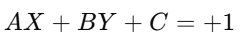
Point Between Hyperplane and Margin (e.g., AX + BY + C = −0.5)

Suppose a red point lies between the hyperplane and the negative margin :

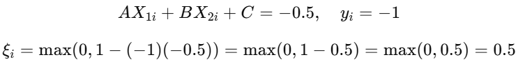
This is a margin violation but not a misclassification. Slack variable is between 0 and 1 .

Misclassified Point (Above Positive Margin)

Now suppose a red point (negative class) lies above the positive margin, say :

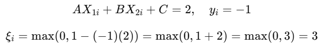
This is a misclassified point, and the hinge loss increases with how far it lies from its correct side .

Hinge Loss Graph

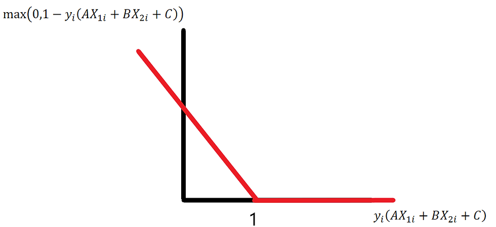
This graph represents how hinge loss penalizes margin violations and misclassifications.

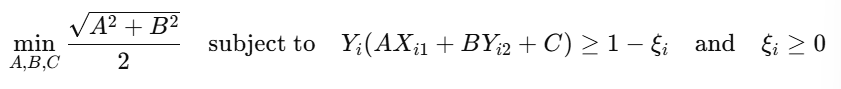
Soft Margin SVM – Concept and Constraints

When we have linearly separable data, we can use the Hard Margin SVM. The optimization problem for that is :

We prefer to rewrite this as a minimization problem, since most loss functions aim to minimize error :

Soft Margin SVM : Introducing Slack Variables

However, when the data is not linearly separable, we relax the constraints using slack variables ξᵢ ≥ 0, which allow for some margin violations. The new formulation becomes :

Key Insight :

This small change (relaxing the margin constraint) allows the model to handle non-linearly separable data by penalizing violations through slack variables.

Testing the Soft Margin Constraint

The new soft margin constraint works well for :

• Points on the correct side of the margin

• Support vectors (points on the margin)

• Points slightly violating the margin

This flexibility is not possible in hard margin SVM, which fails when data is not perfectly separable.

Soft Margin SVM – Flexibility Beyond the Margins

Let’s consider a scenario where our data is not linearly separable, and points do not lie strictly between or outside the SVM margin lines.

Refer to the diagram above. The key lines are :

• Middle line : The decision boundary (model line)

• Dashed lines : Margins

• Green crosses : Class +1 (similar logic applies to red crosses for class -1)

Issue with Hard Margin SVM

In the hard margin SVM, the constraint is :

This requires that all points lie on or beyond the correct margin with no violations. If any point lies between the margin lines or on the wrong side, the constraint fails, and hard margin SVM cannot handle it .

Soft Margin SVM : Updated Constraint

To allow some margin violations, we introduce slack variables ξᵢ , leading to the new constraint :

We can test this constraint on different types of points :

Example 1 : Point between the model line and positive margin line

Assume a point on the line AX + BY + C = 0.5, and it belongs to class Yᵢ = 1 .

True — The constraint holds.

But hard margin SVM would fail here since the point is inside the margin.

Example 2 : Point between model line and negative margin line

Assume a point on the line AX + BY + C = −0.5, and Yᵢ = 1 .

True — The constraint still holds.

Example 3 : Point beyond the negative margin line

Let’s say the point lies on AX + BY + C = −2, and Yᵢ = 1 :

True — Still satisfies the constraint.

Same Logic Applies to Red Points (Class -1)

The inequality generalizes for both classes due to the Yᵢ term. So whether it’s a red or green point, the modified constraint works.

Conclusion : Why Soft Margin Is Powerful

By changing the hard margin constraint to :

we've introduced flexibility. This new condition :

• Allows all points (with some penalty for violations)

• Eliminates strict separability requirements

• Handles real-world noisy data

Thus, the constraint is no longer a rigid condition, but rather a soft condition that adapts to the data. We have dissolved the hard constraint and replaced it with a flexible tolerance using Yᵢ .

Soft Margin SVM – Objective Function and Need for Regularization

We begin by revisiting the updated constraint in soft margin SVM :

Issue with This Formulation

This formulation relaxes the hard margin constraint, allowing some points to :

• Lie inside the margin

• Lie on the wrong side of the decision boundary

While this sounds flexible, without any penalty on the slack variables ξᵢ , this model becomes problematic :

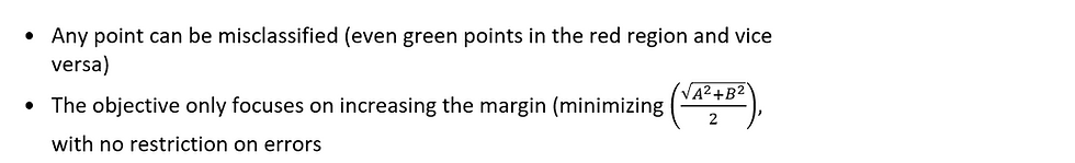
In essence :

The model aims to increase margin without controlling where or how the margins lie, leading to a meaningless or overly flexible solution. The margin can expand indefinitely and fail to align with the data's actual distribution.

Consequences

• We lost logical constraints that define where the margin should stop.

• There is no guarantee that the support vectors (the most critical points) define the margin anymore.

• Misclassifications increase, accuracy drops, and the model fails to generalize well.

This leads to a bad model — we’ve overcorrected by removing too much restriction.

Solution : Add a Penalty for Misclassification

To fix this, we modify the objective function to penalize slack variables :

Interpretation of the Two Terms

Balancing the Trade-Off

• These two terms often conflict :

  • One wants a larger margin (even if some points violate it).

  • The other wants fewer violations (even if it means shrinking the margin).

• Together, they guide the model to a balanced solution :

  • A good-enough margin

  • Controlled misclassifications

This leads to soft margin SVM's core idea : allow some violations, but penalize them appropriately to maintain model performance.

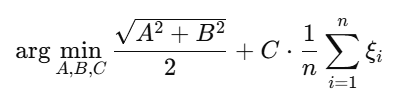
Final Form (with a penalty parameter C) :

More generally, we add a regularization parameter C to control this trade-off :

• Higher C→ prioritize minimizing misclassifications.

• Lower C→ allow more flexibility and a wider margin.

SVM Objective with Hyperparameter C

Subject to :

We introduce a constant C, which is a hyperparameter—its value depends on the data. The value of C is always greater than zero. You can think of C as a tuning knob for the algorithm.

If we increase the value of C too much—for example, to 1000—the algorithm will put a lot of pressure on minimizing the term

This causes the algorithm to focus more on reducing misclassifications, which may lead to narrower margins.

On the other hand, if we reduce the value of C significantly—say to 0.001—then the term

will dominate. The algorithm will then try to maximize the margin between the classes, potentially at the cost of allowing more misclassifications.

By tuning C, we gain control over the balance between maximizing the margin and minimizing classification error.

SVM Parameter C

• In the first diagram with C = 1, the algorithm focuses more on maximizing the margin, even if that allows some misclassifications.

• In the second diagram with C = 100, the algorithm prioritizes reducing misclassifications, resulting in smaller margins but fewer classification errors.

Bias-Variance Trade-off

The value of C plays a crucial role in managing the bias-variance trade-off .

• If C is set too high , the algorithm tries hard to avoid misclassification on the training data. This can lead to overfitting, resulting in low bias but high variance.

• If C is set too low , the algorithm prioritizes increasing the margin, potentially allowing more misclassifications. This may lead to underfitting, resulting in high bias and low variance.

To achieve the best generalization, we must find an optimal value of C that strikes a balance between bias and variance .

RELATIONSHIP WITH LOGISTIC REGRESSION

Drawing Parallels Between SVM and Logistic Regression :

1. In SVM, the term

acts as the loss function, quite similar to the log loss in logistic regression.

2. In Logistic Regression, the regularization term is :

3. In SVM, the regularization term is :

Both are regularization terms, just expressed differently.

Key Insight :

• In logistic regression, λ (lambda) controls the strength of regularization.

• In SVM, C controls the balance between the margin and hinge loss.

Thus, C and λ are inversely proportional :

This relationship reflects that :

• A large C in SVM (less regularization) is like a small λ in logistic regression (also less regularization).

• A small C in SVM (more margin, more regularization) is like a large λ in logistic regression.