Support Vector Machine (SVM) – Part 3

CONSTRAINED OPTIMIZATION PROBLEM

Problem with SVC (Support Vector Classifiers)

Support Vector Machines (SVM) are powerful classifiers that aim to find the optimal hyperplane that best separates different classes in a dataset. There are two main types of SVM :

• Hard Margin SVM : Assumes that the data is perfectly linearly separable. It tries to find a hyperplane that completely separates the classes without any misclassification.

• Soft Margin SVM : Allows some misclassifications by introducing a penalty for errors, making it more flexible and able to handle datasets that are almost linearly separable.

However, both Hard Margin and Soft Margin SVM are fundamentally linear classifiers. This leads to a significant limitation :

If the underlying relationship between the features and the labels is nonlinear, traditional hard margin or soft margin SVMs will still attempt to fit a straight hyperplane, resulting in poor classification performance.

In other words, when facing non-linearly separable data, these linear SVM models cannot find an appropriate decision boundary. They will force a straight line (or hyperplane in higher dimensions) even when a curved or more complex boundary is needed.

Thus, linear SVMs fail on non-linear datasets, and cannot effectively model complex patterns inherent in the data.

Solving the Problem : Introduction to Support Vector Machines (SVMs)

To overcome the limitation of standard Support Vector Classifiers (SVC) on non-linear datasets, we move to the broader concept of Support Vector Machines (SVMs) with Kernels.

• SVC by itself, without kernels, is a linear classifier.

• To handle non-linear data, we introduce the concept of kernels into SVC.

• Kernels transform the original data into a higher-dimensional space where a linear separator (hyperplane) can be found.

• This upgraded approach, where SVC uses kernels to deal with non-linear data, is generally referred to as Support Vector Machines (SVMs).

Thus, SVM = SVC + Kernels (in simple terms).

In summary :

• When kernels are added to the basic SVC, the classifier can effectively handle non-linear datasets.

• This combination is what makes Support Vector Machines (SVMs) a powerful tool for both linear and non-linear classification problems.

Important Points :

• Without kernels : SVC = Linear classifier ➔ Only for linearly separable data.

• With kernels : SVM = Can classify both linear and non-linear data.

Kernels Intuition

1. One-Dimensional Example (Age vs Side Effect)

Suppose we have a simple dataset where :

• Input : Age (feature)

• Output : Side Effect (1 = side effect happened, 0 = no side effect)

Age	Side Effect
72	1
32	0
26	0
5	1

This is a one-dimensional dataset .

Visualization :

When we plot the ages on a number line, we get something like this :

• Red points (×) represent people who experienced side effects (Side Effect = 1).

• Green points (✓) represent people who did not experience side effects (Side Effect = 0).

You can observe :

• At very low and very high ages, side effects happen (red points).

• At middle-range ages, side effects do not happen (green points).

Problem with SVC :

• If we apply a basic Support Vector Classifier (SVC) here, it will try to separate the classes linearly.

• In 1D, SVC can only select a threshold point to separate the data.

• However, here the red and green points are intermixed — so no single point can perfectly separate them.

Conclusion :

A simple linear SVC fails to classify such non-linearly separable data.

2. Two-Dimensional Example (Center Green, Surrounding Red)

Now, let's take another situation :

Imagine a 2D dataset where :

• The green points (no side effect) are clustered in the center.

• The red points (side effect) surround the green points in a circular fashion.

Problem with Linear SVC in 2D :

• We are asked to draw a straight line to classify the points.

• But no straight line can separate the center green points from the surrounding red points!

• Whatever line we draw, it will always misclassify some points.

Thus, linear SVC fails again.

In these types of non-linear situations, we apply Kernel methods.

Kernels help SVM solve non-linear classification problems by mapping the data into a space where classes become linearly separable.

Understanding Kernels and How They Work

What are Kernels ?

In simple words :

Kernels are mathematical functions that transform input data into a higher-dimensional space.

The idea behind kernels is to make data that is not linearly separable in its original dimension become linearly separable in a higher dimension.

How Kernels Work (Step-by-Step) :

1. Start with the original data :

• In the first example we discussed earlier, the data was one-dimensional (Age vs Side Effect).

• In the second example, the data was two-dimensional (center green points surrounded by red points).

2. Apply a Kernel Function :

• The kernel function transforms the data into a higher-dimensional space.

• Example :

  • 1D data ➔ Transformed into 2D space.

  • 2D data ➔ Transformed into 3D space.

3. Why Transform ?

• Kernel functions are carefully designed so that in the higher-dimensional space, the data becomes linearly separable.

• This means classes can be separated using a straight line (hyperplane) in the higher dimension.

4. Apply SVM or SVC :

• In this higher-dimensional space, we apply the Support Vector Machine (SVM) or Support Vector Classifier (SVC).

• Now, because the data is linearly separable, SVM can find an optimal hyperplane that perfectly separates the classes.

5. Project Back to the Original Space :

• Once the decision boundary (the separating hyperplane) is found in the higher-dimensional space, we bring the result back into the original lower-dimensional space.

• In the original space, the decision boundary appears as a curve or a non-linear boundary, achieving non-linear classification.

Final Intuition :

Kernels let SVM solve non-linear problems by temporarily moving the data into a higher dimension where it becomes easy to separate, then bringing the result back down.

Quick Summary :

Step	Action
1	Start with original data (possibly non-linear)
2	Apply Kernel function to transform data into higher dimension
3	In higher dimension, data becomes linearly separable
4	Apply SVM/SVC to find the separating hyperplane
5	Bring decision boundary back to original dimension (resulting in non-linear separation)

 Here are the main types of kernels used in SVM :

Why Is It Called the Kernel Trick ?

We call it a "trick" because :

1. We avoid explicitly transforming data to higher dimensions.

Normally, to make non-linearly separable data linearly separable, we would transform the data into a higher-dimensional space (e.g., going from 1D to 2D, or from 2D to infinite dimensions using RBF kernel). But doing this explicitly is computationally expensive.

2. The trick is : we don’t actually do the transformation.

   
   

Instead, we compute the dot product between data points as if they were in that higher-dimensional space — using a kernel function.

3. It reduces computation and memory use .

This lets us run complex algorithms as if they were working in a high-dimensional space, while still working in the original (lower) dimensional space.

So What’s the Trick ?

• The trick is mathematical : instead of explicitly computing in high dimensions, we cleverly compute the result using kernel functions that simulate the effect of working in that high-dimensional space.

• The benefit is efficiency : we get the power of high-dimensional classification without paying the computational cost of going there.

 Summary

We call it a "trick" because we don't actually transform the data into a higher dimension — we pretend as if we did, by using a kernel function that computes inner products as though the transformation happened. This way, we save memory, reduce computation, and still classify data that was not linearly separable before. That’s the beauty of the kernel trick — it’s smart math, not brute force.

Example 1 : Age vs. Side Effect

Suppose we are analyzing the relationship between a patient's age and whether they experience a side effect (yes/no). Imagine that our data is plotted on a 1D axis where :

• Red  marks indicate side effects occurred

• Green  marks indicate no side effects

This data is clearly not linearly separable in one dimension. A straight line cannot distinguish red from green points effectively.

Applying a Kernel (Non-Linear Transformation)

To separate the data, we apply a kernel transformation. In this example, we use a kernel that maps the input x to x² . This transforms our 1D data into a 2D space :

• The x-axis remains as x

• The y-axis becomes x²

Now in this 2D space, the data becomes linearly separable, and we can draw a straight line (a linear decision boundary) that separates the red and green points.

Example 2 : Circular Distribution

In a second example, consider data points arranged in a circular pattern :

• The green points are at the center

• The red points form a ring around them

This pattern is again not linearly separable in 2D. No straight line can divide the green and red points .

Applying a Kernel : Moving to 3D

We now use a radial basis function–style kernel, such as :

                                     z = x₁² + x₂²

This transformation projects the data into 3D space :

• x₁ and x₂ are retained as input axes

• z = x₁² + x₂² is the new third axis (height)

In this 3D representation :

• Points with higher x₁² + x₂² (the red ring) are mapped higher along the z-axis.

• Points with lower values (green center) are mapped lower along the z-axis.

This makes it possible to draw a flat plane (hyperplane) in 3D to separate the two classes. Then, we project this hyperplane back into 2D to get a non-linear decision boundary in the original input space.

Intuition Behind the Kernel Trick

In simple terms :

• The kernel trick allows us to transform data into higher dimensions, where it becomes linearly separable.

• In that higher-dimensional space, we apply a linear SVM, find the optimal hyperplane, and then project it back to the original space.

• This gives us a non-linear decision boundary in the original feature space, enabling SVM to handle complex patterns effectively.

Why Is It Called a "Kernel Trick" ?

The term "kernel trick" is used because it's not just a straightforward transformation—it's a clever mathematical shortcut.

At first glance, it seems like we are transforming the data into a higher-dimensional space (e.g., from 2D to 3D) to make it linearly separable. But here's the trick :

• We do not explicitly compute the coordinates of the data in that higher-dimensional space.

• Instead, we use a kernel function to compute the inner product between pairs of data points as if they were in that higher-dimensional space.

This allows the SVM to operate implicitly in a higher dimension, while performing all computations in the original (lower-dimensional) space. This avoids the cost of actually computing and storing high-dimensional vectors.

So what's the "trick" ?

• The trick is that we get the benefits of high-dimensional transformations without ever performing them explicitly .

• This reduces computational cost, saves memory, and makes the algorithm faster and more scalable .

Summary

We call it a trick because :

• It feels like we are transforming the data to a higher dimension (to make it separable),

• But in reality, we don't—we stay in the original space and simulate the effect of that transformation using a kernel function.

• The whole process is mathematically elegant, efficient, and avoids high-dimensional computation.

That’s the beauty of the kernel trick—a smart mathematical workaround that gives us powerful results with lower cost .

Mathematics of SVM – Understanding Constrained Optimization

To understand the mathematics behind Support Vector Machines (SVM), we first need to grasp constrained optimization.

Optimization Recap

In previous topics like Linear Regression and Logistic Regression, we also solved optimization problems. There, the goal was to minimize a loss function by finding the best values for the model's coefficients (like weights or betas). For example :

• In linear regression : minimize the mean squared error.

• In logistic regression : minimize the log-loss.

This involves using methods like OLS or gradient descent, and we often calculate derivatives to find the optimal values that minimize the loss.

What is Constrained Optimization ?

In constrained optimization, the objective remains the same (minimize or maximize a function), but now there's a condition (called a constraint) that must be satisfied.

This makes the problem harder : we can't just minimize any function—we have to find a minimum within a feasible region defined by the constraint.

SVM's Constrained Optimization Problem

SVM tries to find the optimal hyperplane that separates two classes. Mathematically, it tries to :

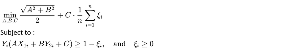
Here :

• A , B , C define the hyperplane (decision boundary).

• ξᵢ are slack variables (they allow some misclassifications).

• The constraint ensures that all points lie on the correct side of the margin or have a penalty via ξᵢ .

The goal is to minimize the margin width and penalty for misclassification together.

A Simple Constrained Optimization Example

To understand constrained optimization intuitively, consider the problem :

This means : find the values of x and y that maximize x²y, but only among those that satisfy the constraint x² + y² = 1 .

Invalid Example :

If you choose x = 5 , y = 7, then :

        x² + y² = 25 + 49 = 74   (does not satisfy the constraint)

So these values are not allowed.

Valid Example :

This is a valid solution—it satisfies the constraint and gives a function value.

The challenge is that there are many combinations of x and y that satisfy the constraint. The goal is to find the one that gives the maximum value for the objective function while still satisfying the constraint.

Summary

• Unconstrained optimization : minimize the function freely.

• Constrained optimization : minimize (or maximize) the function but within limits.

• SVM uses constrained optimization to find the best separating hyperplane while penalizing misclassifications using slack variables.

Geometric Intuition Behind Constrained Optimization (Foundation for SVM)

In Support Vector Machines (SVM), optimization under constraints is central. To build strong intuition for how this works, let’s begin with a simpler constrained optimization problem and visualize it geometrically. This will help us understand why SVM’s objective (maximizing margin subject to constraints) is formulated the way it is.

The Problem Setup

We are given the following optimization problem :

Let’s unpack this :

• The objective function f(x , y) = x²y is what we want to maximize.

• The constraint x² + y² = 1 restricts the values that x and y can take — only points that lie on the unit circle in the xy-plane are allowed.

Step 1 : Visualizing the Objective Function in 3D

Since f(x,y) is a function of two variables, it forms a 3D surface in space. We can imagine this as a “hill” or “valley” depending on the shape of the function. Each point on the surface has coordinates (x,y,z) , where z = x²y .

This surface bends and curves depending on the values of x and y. Some parts rise above the plane (positive z), some dip below (negative z), depending on the sign and magnitude of y.

Step 2 : Visualizing the Constraint — The Unit Circle

The constraint x² + y² = 1 defines a circle in the xy-plane. We are only allowed to pick points on this circle when choosing x and y.

Imagine slicing the 3D surface of the function with a vertical wall that traces this circle. What do we get ?

Step 3 : Mapping the Circle Onto the Surface

Take every point (x, y) on the circle x² + y² = 1 , and plug it into the function f(x,y) =x²y . This gives us a new set of 3D points (x ,y , x²y), which trace out a curve on the surface of the function.

This curve represents all possible function values subject to the constraint. Our task now is to find the highest point on this curve — that’s the solution to our optimization problem.

Step 4 : From 3D Surface to 2D Contour Plot

Working in 3D is hard. To simplify, we often use a contour plot, which is a 2D projection of the 3D surface :

• Contour lines represent constant values of f(x,y) (i.e., constant z-levels).

• Closer contours mean the function is changing rapidly.

• Brighter or more intense regions (e.g., yellow) indicate higher values of z.

On this plot :

• The circle shows all valid (x,y) pairs (our constraint).

• The contour lines represent increasing or decreasing values of the function.

Step 5 : Interpreting Contours and Constraints Together

Now comes the key idea :

• Each contour line represents a fixed value of the function (a specific height).

• We want to find the highest contour line that still touches the constraint circle.

Let’s say the yellow area corresponds to a contour line where f(x, y) = 0.2, and it intersects the circle in two places. These points satisfy the constraint and give us a valid z = 0.2.

But what if there's another contour, say z = 0.4, that also intersects the circle ? Then that gives us a better (higher) solution.

Now imagine a contour z = 4 — it might not intersect the circle at all. That means those values of x and y don’t satisfy the constraint .

The highest contour that just touches the constraint is our optimal solution. This is the point at which the gradient of the function is aligned with the gradient of the constraint — a condition formalized by Lagrange multipliers.

Conceptual Summary

• The 3D surface of f(x,y) shows how function values change in space.

• The constraint circle restricts us to a path along that surface.

• By projecting the surface to a 2D contour plot, we visualize the optimization as finding the highest contour that intersects the constraint.

• The solution occurs where a contour line is tangent to the constraint curve.

This exact idea — maximizing a quantity under a constraint — is what happens in SVM :

• We maximize the margin (analogous to z = f(x,y) )

• Subject to classification constraints (analogous to the circle)

Bonus Insight : Symmetry in the Problem

Because both the function f(x, y) = x²y and the constraint x² + y² = 1 are symmetric, we often get more than one optimal point — mirrored across axes. This is not a failure but a feature of the problem’s structure.