Support Vector Machine (SVM) – Part 7

Aryan
May 8
7 min read

Understanding Local Decision Boundaries with RBF Kernel

Suppose we have red and green data points in space, as shown in the image. These points form clusters or regions of influence around them.

How the Kernel Defines Region of Influence

Each point influences its neighborhood through the RBF kernel function :

The similarity (kernel value) decreases exponentially with distance.
Only nearby points have significant similarity.
Every point effectively forms a "soft boundary" around itself — a region where it dominates the classification.

What Happens When Classes Mix ?

When red and green points are well-separated, their respective regions are also separate.
If red and green points intermingle, their regions overlap.
This overlap leads to a complex and curved decision boundary — it no longer looks like a straight line or simple curve.

Why It’s Called a Local Decision Boundary

The RBF kernel creates local effects — a point influences only its close neighbors.
If a new data point falls within a red region, it’s classified as red; if it’s within green, it's classified as green.
If it falls outside any region, it’s classified based on the nearest influence.

This locality means decision boundaries are flexible and adaptive — perfect for non-linear data.

RBF kernels create local decision regions by assigning high similarity only to nearby points.
The decision boundary is shaped by the arrangement of data points and the exponential decay of the kernel function.
This leads to complex, highly non-linear decision boundaries, which is a major strength of kernelized SVMs.

Effect of Gamma

The parameter γ in the Radial Basis Function (RBF) kernel of a Support Vector Machine (SVM) is a hyperparameter that determines the spread of the kernel and therefore the decision region.

The effect of γ can be summarized as follows :

If γ is too large, the exponential will decay very quickly, which means that each data point will only have an influence in its immediate vicinity. The result is a more complex decision boundary, which might overfit the training data.
If γ is too small, the exponential will decay slowly, which means that each data point will have a wide range of influence. The decision boundary will therefore be smoother and more simplistic, which might underfit the training data.

In a sense, γ in the RBF kernel plays a role similar to that of the inverse of the regularization parameter: it controls the trade-off between bias (underfitting) and variance (overfitting). High γ values can lead to high variance (overfitting) due to more flexibility in shaping the decision boundary, while low γ values can lead to high bias (underfitting) due to a more rigid, simplistic decision boundary.

Tuning the γ parameter using cross-validation or a similar technique is typically a crucial step when training SVMs with an RBF kernel.

Understanding the RBF Kernel Geometrically

Let’s understand the Radial Basis Function (RBF) kernel with the help of diagrams and an intuitive explanation.

The RBF kernel formula is :

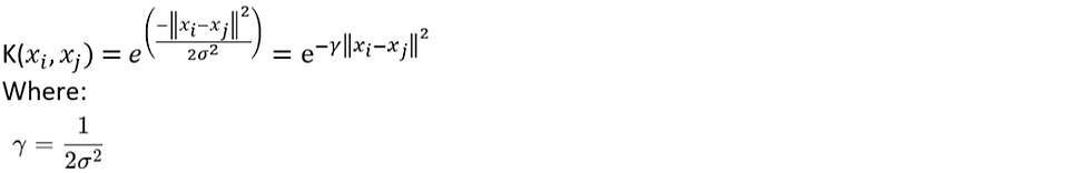
Here, σ controls the spread or width of the kernel function and γ is its inverse scaling.

Visualizing Different Values of σ

We can visualize how the kernel behaves with different values of σ by plotting the exponential function for varying σ. This will show how the similarity measure decays as the distance ||xᵢ − xⱼ|| increases.

In the graph above, each curve represents a different value of σ. As σ increases, the kernel becomes wider and flatter. Conversely, as σ decreases, the kernel becomes sharper and narrower.

Effect of σ on Locality and Similarity

σ² appears in the denominator of the exponent, similar to its role in a Gaussian (normal) distribution. It controls the width of the graph, which determines how far the "similarity" extends :

If σ is large, the width of the kernel function increases. This means that even distant points are considered similar, making the kernel more accommodating.
If σ is small, the width decreases sharply, and only very close points are considered similar. This increases locality and reduces generalization.

Controlling the Locality with σ

Using σ , we can control how "local" the influence of a data point is:

High σ → Broad region of influence → Points far apart can still be considered similar → Risk of underfitting.
Low σ → Narrow region of influence → Only very close points are similar → Risk of overfitting.

So, σ acts as a hyperparameter that controls the locality of the model.

Relationship Between σ and γ

Since :

Increasing γ reduces σ , making the model more local.
Decreasing γ increases σ , making the model more global.

Bias-Variance Tradeoff

There is a tradeoff between bias and variance when choosing σ :

Small σ (large γ ) : The model becomes highly sensitive to nearby points, resulting in high variance and low bias → risk of overfitting.
Large σ (small γ ) : The model generalizes over larger distances, resulting in low variance and high bias → risk of underfitting.

Relation Between RBF and Polynomial Kernel

Infinite Dimensional Mapping :

The RBF kernel implicitly maps input data to an infinite-dimensional feature space, allowing for even greater flexibility in forming decision boundaries.

Conceptual Understanding

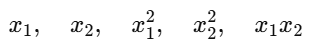
If we consider a polynomial kernel, suppose we have two features x₁ and x₂ .

Applying a second-degree polynomial gives :

But the RBF (Radial Basis Function) kernel can implicitly generate infinitely many polynomial terms between these points.

So not only does it include :

It also includes all terms of degree 3, 4, 5, and so on.

This means it effectively maps the data from 2D to an infinite-dimensional feature space.

In a polynomial kernel, we manually construct vectors like 6D, treating them as fixed-dimensional.
In contrast, the RBF kernel has the power to transform data into an infinite-dimensional vector that includes all possible polynomial terms.

Why is this powerful ?

Because with all possible polynomial terms, the function can form any curve, fit any complex pattern, and create highly flexible decision boundaries.

That’s why the RBF kernel is said to have the universal approximation property.

The Radial Basis Function (RBF) kernel is defined as :

For some temporary simplification, let's set σ = 1 . This is for mathematical convenience during the derivation and the general form can be recovered later.

Conceptual Understanding :

This derivation reveals a powerful property of the RBF kernel. By mapping data into an infinite-dimensional feature space where the coordinates relate to polynomial expansions of the original features, the RBF kernel implicitly performs classification or regression using features equivalent to all orders of polynomial combinations of the original input features. This is why the RBF kernel is considered highly flexible and is often referred to as a "universal kernel" – it can implicitly model highly complex, non-linear relationships in the data without explicitly computing these high-dimensional features. This ability to work in an infinite-dimensional space implicitly is a key aspect of the "kernel trick".

Custom Kernels

String kernels : These are used for classifying text or sequences, where the input data is not numerical. String kernels measure the similarity between two strings. For example, a simple string kernel might count the number of common substrings between two strings.
Chi-square kernel : This kernel is often used in computer vision problems, especially for histogram comparison. It’s defined as

where χ²(x,y) is the chi-square distance between the histograms x and y.

Intersection kernel : This is another kernel commonly used in computer vision, which computes the intersection between two histograms (or generally non-negative feature vectors).

Hellinger’s kernel : Hellinger’s kernel, or Bhattacharyya kernel, is used for comparing probability distributions and is popular in image recognition tasks.

Radial basis function network (RBFN) kernels : These are similar to the standard RBF kernel, but the centers and widths of the RBFs are learned from the data, rather than being fixed a priori.
Spectral kernels : These kernels use spectral analysis techniques to compare data points. They can be particularly useful for dealing with cyclic or periodic data.

Support Vector Regression (SVR)

Dataset and Problem Context

Suppose we have a dataset where :

X-axis = House Size
Y-axis = House Price

Our goal is to predict the price of a house based on its size. SVR helps us fit a regression model with maximum margin around the predicted line while allowing some flexibility for errors.

Constructing the SVR Model Line and Margin (ε-tube)

In SVR, we start by creating a best fit model line represented as :

Let’s simplify by assuming b=0, so it becomes :

To handle real-world data that may not perfectly lie on this line, we introduce a margin of tolerance (epsilon, ε). This creates a tube or band around the line.

The upper margin line becomes :

The lower margin line becomes :

This zone between the two margins is called the ε-tube. Points lying within this tube are considered correct predictions, and we do not penalize them.