What is an MLP? Complete Guide to Multi-Layer Perceptrons in Neural Networks

Aryan
7 days ago
9 min read

THE PROBLEM: Limitations of a Single Perceptron

The fundamental issue with a single perceptron is its inability to solve problems involving non-linear data.

The Limitation: A perceptron creates only a straight line (a linear decision boundary) to separate data points into different classes.
The Consequence: As shown in the example image , we have two classes (red and green) that cannot be perfectly separated by a single straight line. This is called non-linearly separable data.
The Goal: We need to develop an algorithm, built upon the concept of the perceptron, that can capture this non-linearity and produce a curved decision boundary (or a set of linear boundaries that collectively form a non-linear one) to effectively classify the data.

PERCEPTRON WITH SIGMOID

In this section, we use a perceptron whose activation function is sigmoid instead of a step function. The loss function used is log loss, making it conceptually similar to logistic regression.

Let’s understand how it works with the sigmoid function.

Suppose we have two input features — CGPA and IQ — and our task is to predict placement.

In a sigmoid-based model, the output is not 0 or 1 (as in a step function), but a probability between 0 and 1, which represents how likely the student is to be placed.

Assume we train the model and obtain parameters:

w₁ = 5, w₂ = 10, b = 3

The equation of the decision boundary is:

5x + 10y + 3 = 0

For a new student with CGPA = 8.7 and IQ = 87, we calculate

z = 5x + 10y + 3

and pass this value through the sigmoid function,

to obtain a probability between 0 and 1.

If the output is 0.8, it means the probability of placement is 0.8 (and not being placed is 0.2).

Each point in the dataset represents a student. The decision boundary (the line) divides the region into two parts.

Students lying on the line have a 0.5 probability — equal chances of being placed or not.
As we move further from the line into the green region, the probability of placement increases (e.g., 0.6 → 0.8 → 0.9).
Conversely, moving further into the red region increases the probability of not being placed.

Thus, the sigmoid activation allows us to interpret model outputs as probabilities, capturing a smooth transition between classes rather than a hard boundary.

FORMING IDEA OF MLP

Let’s try to form an intuition for a Multi-Layer Perceptron (MLP).

Suppose we have two perceptrons:

For the first perceptron: w₁ = 2, w₂ = 3, b = 6 → decision boundary: 2x + 3y + 6 = 0
For the second perceptron: w₁ = 5, w₂ = 4, b = 3 → decision boundary: 5x + 4y + 3 = 0

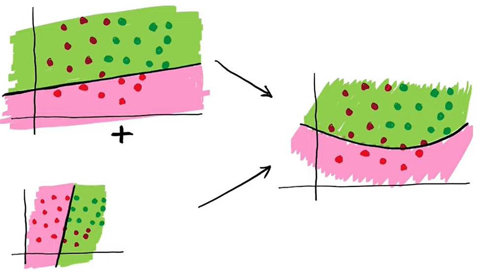
Now, if we combine (add) the results of both perceptrons, we can visualize the two decision boundaries on the same plot.

Think of it as superimposing two images — each representing a perceptron’s line — and then performing a kind of smoothing operation over them. The result is a curved or blended boundary, which represents a more flexible decision surface.

This gives us the abstract idea of a multi-layer perceptron:

We combine the outputs of multiple perceptrons, and through this aggregation and smoothing, the model can learn non-linear boundaries that a single perceptron could never capture.

MATHEMATICS BEHIND MLP

All these points on the plot represent data points.

Let’s take a simple analogy — suppose each point represents a student from the green region.

According to the first perceptron, this student has a 0.7 probability of being placed.
According to the second perceptron, the probability is 0.8.

Each student (data point) therefore gets a placement probability from both perceptrons.

Now, to combine these two perceptrons, we simply add their output probabilities:

0.7+0.8 = 1.5

But this value (1.5) doesn’t make sense as a probability — it exceeds 1.

So, we pass it through a sigmoid function, which compresses the value into a valid probability range between 0 and 1:

σ(1.5) = 0.82

Hence, the combined model now gives a probability of 0.82 for this student being placed.

We repeat the same process for every data point — add the perceptron outputs, pass them through the sigmoid, and get the final probabilities.

In this way, we’ve effectively combined multiple perceptrons to build a new model capable of handling more complex (non-linear) patterns.

EXTENDING THE CONCEPT: LINEAR COMBINATION OF TWO PERCEPTRONS

Now, suppose we want a different decision boundary — one where the first perceptron has a stronger influence than the second.

Can we modify our model so that one perceptron’s output dominates the other?

Yes, we can — by introducing weights.

Earlier, we were adding the perceptron outputs directly before applying the sigmoid.

Now, instead of simple addition, we’ll do a weighted addition — assigning a weight to each perceptron’s output based on its importance.

Let’s assume:

Weight of Perceptron 1 = 10
Weight of Perceptron 2 = 5

If Perceptron 1 gives 0.7 and Perceptron 2 gives 0.8, the weighted sum becomes:

z = (0.7 × 10) + (0.8 × 5) = 11

If we also add a bias term, say 3, we get:

z = (0.7 × 10) + (0.8 × 5) + 3 = 14

We then pass this value through the sigmoid function to obtain the final probability:

P=σ(14)

This process is repeated for every data point, giving us probabilities between 0 and 1 for each student.

Essentially, this setup behaves like a new perceptron — but one that takes as input the outputs of other perceptrons.

So, what we’ve done is stacked perceptrons:

The first layer produces outputs (0.7, 0.8, etc.)
The second layer takes those as inputs, applies weights and bias, and generates final probabilities.

This architecture — where outputs of perceptrons become inputs to another perceptron — is known as a Multi-Layer Perceptron (MLP).

BUILDING THE FINAL MULTI-LAYER PERCEPTRON (MLP)

On the left side, we have our two perceptrons, and on the right side, we have their linear combination.

We’re working with student data — say CGPA, IQ, and whether the student is placed or not placed.

The two perceptrons can be represented by the following equations:

Perceptron 1: 2x + 3y + 6 = 0

Perceptron 2: 5x + 4y + 3 = 0

Here,

CGPA and IQ are the inputs.
The first perceptron has a bias = 6, and the second has a bias = 3.
At the combined perceptron, we assign weights — 10 for the first perceptron’s output and 5 for the second’s.

So, we first compute the outputs (z-values) from both perceptrons and then combine them linearly using these weights.

The third perceptron then takes these combined outputs as its inputs and has its own bias of 3.

This third perceptron produces the final prediction (e.g., probability of being placed).

Network Representation

We can visualize or redraw it as:

Or more clearly in layer form:

Input Layer: CGPA, IQ
Hidden Layer: Two perceptrons (with biases 6 and 3)
Output Layer: Third perceptron (with bias 3)

Final Concept

This setup is called a Multi-Layer Perceptron (MLP) — it has:

An input layer
A hidden layer
An output layer

By combining multiple perceptrons in this way, we can capture non-linearity in the data.

In essence, we’re making linear combinations of multiple perceptrons, stacking them to create a model that can learn complex, curved decision boundaries that a single perceptron could never form.

ADDING NODES IN HIDDEN LAYER

In this section, we’ll learn how to modify the architecture of a neural network to make it more flexible.

The architecture of a neural network refers to how nodes (or perceptrons) are connected — the structure of inputs, hidden layers, outputs, and weights between them.

We can modify this architecture depending on the complexity of data and our model requirements.

1. Increasing Nodes in the Hidden Layer

In our example, we currently have three perceptrons in the hidden layer.

If our data is highly non-linear, increasing the number of perceptrons allows the model to capture more non-linearity.

By merging the outputs of these perceptrons, we can form more complex curved decision boundaries.

This works similarly to the two-perceptron case we studied earlier — adding more perceptrons simply introduces more terms in the overall equation, helping the model form richer and more flexible boundaries.

In short:

More perceptrons → More terms in the equation → More ability to model non-linear patterns.

2. Increasing Nodes in the Input Layer

Sometimes, we add new features to our dataset — for example, suppose in addition to CGPA and IQ, we also include a student’s 12th-grade marks.

Now our data moves from 2D to 3D space.

X-axis → CGPA
Y-axis → IQ
Z-axis → 12th marks

Each perceptron now forms a plane instead of a line.

We can combine (linearly or non-linearly) these planes using weights and biases, then pass the combined value z through the sigmoid function to get a probability between 0 and 1.

This is how we extend our model to handle higher-dimensional data by increasing input nodes.

3. Increasing Nodes in the Output Layer

So far, we have used one output perceptron, which suits binary classification (e.g., placed/not placed).

However, for multi-class classification, we need multiple output nodes.

For example:

Classifying an image as dog, cat, or human → requires 3 output perceptrons, one for each class.

Each output perceptron gives the probability that the input belongs to that specific class.

This is a common setup for multi-class classification tasks.

4. Deep Neural Networks (Increasing Hidden Layers)

Another way to modify architecture is by increasing the number of hidden layers, creating what we call a Deep Neural Network (DNN).

Having multiple hidden layers allows the network to:

Capture complex, non-linear relationships in data
Learn hierarchical patterns
Act as a universal function approximator

The idea is simple:

With enough hidden layers and training time, a neural network can approximate any complex mathematical function.

Adding more hidden layers improves the network’s ability to handle intricate data patterns, making it ideal for real-world, high-dimensional problems.

Architectural Change	Purpose
Increase Hidden Nodes	Capture more non-linearity and flexible boundaries
Increase Input Nodes	Incorporate more features (higher-dimensional data)
Increase Output Nodes	Enable multi-class classification
Increase Hidden Layers	Build deeper networks for complex data

MLP Notation

In this section, we’ll learn how to interpret a neural network’s architecture and count the number of trainable parameters (weights and biases).

By examining the architecture, we can calculate:

How many weights and biases exist, and
How to represent them mathematically using standard MLP notation.

Understanding the Architecture

In the diagram above, we have a neural network with four layers:

Input layer (Layer 0)
Hidden layer 1 (Layer 1)
Hidden layer 2 (Layer 2)
Output layer (Layer 3)

Our dataset has four input features and one output feature.

Before training, we can already determine the total number of trainable parameters (weights + biases).

Counting Trainable Parameters

Let’s count step by step:

Between Input Layer and Hidden Layer 1:
- 4 inputs × 3 neurons = 12 weights
- 3 biases (one per neuron)
  → Total = 15 parameters
Between Hidden Layer 1 and Hidden Layer 2:
- 3 inputs × 2 neurons = 6 weights
- 2 biases
  → Total = 8 parameters
Between Hidden Layer 2 and Output Layer:
- 2 inputs × 1 neuron = 2 weights
- 1 bias
  → Total = 3 parameters

Total trainable parameters = 15 + 8 + 3 = 26

When we train this neural network, the backpropagation algorithm will update these 26 parameters to minimize the loss.

Notations for Weights, Biases, and Outputs

Let’s learn how to represent each component mathematically.

1. Biases

Denoted as bᵢⱼ,
where:
- i → layer number
- j → node number in that layer

Example:

b₁₁ → bias of the 1st neuron in Layer 1
b₂₂ → bias of the 2nd neuron in Layer 2

2. Outputs

Denoted as Oᵢⱼ,
where:
- i → layer number
- j → node number

Example:

O₁₁, O₁₂, O₁₃ → outputs from 3 neurons in the first hidden layer
O₂₁, O₂₂ → outputs from neurons in the second hidden layer
O₃₁ → final output neuron (our prediction)

3. Weights

Denoted as wᵏᵢⱼ or wᵢⱼ⁽ᵏ⁾,
where:
- i → node number in the current layer
- j → node number in the next layer
- k → layer index indicating the connection between layers k and k+1