DECISION TREES - 3

Feature Importance in Decision Trees

Feature importance in a decision tree reflects how much a given feature contributes to reducing impurity (e.g., Gini or entropy). It is computed as the normalized total reduction of the criterion (like Gini impurity or entropy) brought by that feature over all the nodes where the feature is used to split.

This is also referred to as Gini importance.

Mathematical Formula

The feature importance for a feature k is defined as :

Where:

• nⱼ is the importance of node j (typically measured by the decrease in impurity weighted by the number of samples that reach the node).

• The numerator sums over nodes where feature k is used.

• The denominator sums over all nodes.

Practical Interpretation

In tree-based algorithms like Decision Trees, Random Forests, or Gradient Boosted Trees, the model automatically calculates feature importances during training. You can access them in scikit-learn using :

model.feature_importances_

This value helps in feature selection by identifying which features contribute most to decision making.

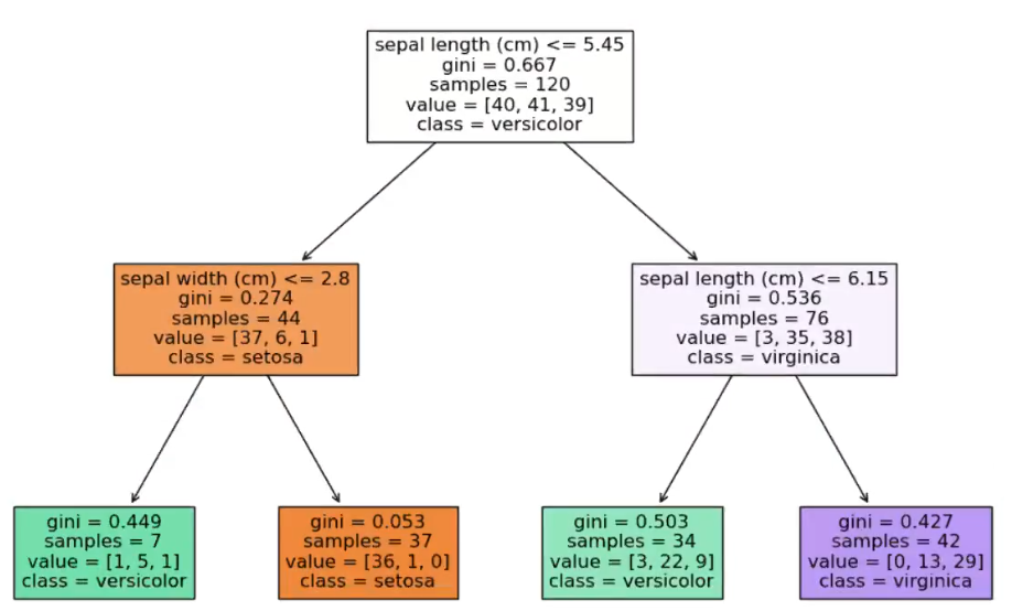
Example : Depth-2 Tree with Iris Dataset Features

Let’s suppose we build a decision tree of depth = 2 trained on the Iris dataset. The splits are :

• Root node: split based on sepal length

• Left child node: split based on sepal width

• Right child node: again split on sepal length

Let the impurity reduction (importance) at each node be :

• Root (node 0, sepal length): x

• Left child (node 1, sepal width): y

• Right child (node 2, sepal length): z

Then, the total importance sum = x + y + z

Summary

• Decision Trees assign importance to features based on how much they reduce impurity.

• The more a feature is used to make splits that reduce impurity, the higher its importance.

• Feature importances are useful for interpretability and feature selection.

Node Importance Calculation

How do we calculate the importance of a node ?

To compute the node importance, we use the following formula :

Step-by-Step Calculation Using Example

We are given the following :

• Root node (parent) :

  • Samples = 120

  • Gini impurity = 0.667

• Right child :

  • Samples = 76

  • Gini impurity = 0.536

• Left child :

  • Samples = 44

  • Gini impurity = 0.274

Now, apply the formula :

Or as calculated explicitly :

This value (≈ 0.2285) is the importance score of the root node, indicating how much it contributes to reducing the impurity in the tree. This node importance is later used to compute feature importance by aggregating the node importances across the tree where a feature is used for splitting.

Node : sepal width (cm) <= 2.8

• Gini impurity = 0.274

• Samples = 44

• Left child :

  • Samples = 7

  • Gini = 0.449

• Right child :

  • Samples = 37

  • Gini = 0.053

Using the formula :

Plug in the values :

Node importance = 0.05938

Node : sepal length (cm) <= 6.15

• Gini impurity = 0.536

• Samples = 76

• Left child :

  • Samples = 34

  • Gini = 0.503

• Right child :

  • Samples = 42

  • Gini = 0.427

Apply the same formula :

Node importance = 0.0475

After calculating node importance for each split in the tree, feature importance is computed by summing up the node importances for each feature and normalizing over all node importances.

Step-by-step :

We already computed :

• Node importance for :

  • Root node (split on sepal length) = 0.22853

  • Right child of root (split on sepal length) = 0.0475

  • Left child of root (split on sepal width) = 0.05938

Feature Importance Formula:

For sepal length :

For sepal width :

Final Results :

Feature	Importance
Sepal Length	0.82296
Sepal Width	0.17704

 The values sum up to 1, which confirms the correctness of normalization.

Interpretation :

• Sepal length is the more important feature in this tree — it contributes to most of the reduction in Gini impurity.

• Sepal width is less important but still contributes meaningfully.

THE PROBLEM OF OVERFITTING

Overfitting in Decision Trees (Classification Case)

In classification problems, decision trees aim to perfectly classify every training instance. This often leads to a problem called overfitting, where the tree becomes overly complex and sensitive to noise in the data.

For example, imagine a binary classification task with two classes: green and purple. Suppose there are a few misclassified points — say, a single purple point in an otherwise green region, or a green point in a purple region. A decision tree will attempt to split again and againjust to correctly classify these outliers.

This behavior results in very narrow and irregular decision boundariesthat are tailored to the training set. These boundaries create small "islands" of one class within regions dominated by another, purely to accommodate those few misclassified examples.

In doing so, the tree "tries too hard to make the training dataset happy," sacrificing its ability to generalize to new, unseen data. This leads to poor performance on the test set, even though training accuracy might be 100%.

This is a classic symptom of overfitting — the model captures noiseinstead of the underlying patterns.

Overfitting in Decision Trees (Regression Case)

Just like in classification, decision trees used for regressioncan also suffer from overfittingwhen they try too hard to perfectly fit the training data.

In regression trees, the input space is split into regions, and each region is assigned a constant output value, typically the mean of the target valueswithin that region. If the tree is allowed to grow without any restrictions (like depth limit or minimum samples per leaf), it may end up creating a separate region for every single data point.

This results in a piecewise constant function that tries to touch every point in the training set, including outliers. While this can lead to very low training error— possibly even zero — the model is capturing not just the true trend, but also the noise in the data.

As a result, the regression tree performs poorly on new data, because it lacks the ability to generalize. This is a classic case of overfitting.

Key Characteristics of Overfitting in Regression Trees

• Highly irregular prediction curves (e.g., a step function with many sharp jumps).

• Extremely low training error but high test error.

• Sensitive to outliers and minor fluctuations in the training data.

To prevent this, we typically apply regularization techniques, such as:

• Limiting tree depth

• Setting a minimum number of samples per leaf

• Pruning

• Using ensemble methods like Random Forest or Gradient Boosted Trees

Why So Much Overfitting Happens in Decision Trees

Decision trees naturally tend to overfitdue to the way they are built. Their default behavior aims to fit the training data as closely as possible — often too closely.

Core Reason : Splitting Until Perfection

Classification Case :

• When constructing a decision tree for classification, the goal is to split the data so that each region (or leaf node) contains samples from only one class.

• The tree keeps splitting the data recursively, creating smaller and smaller regions, until it achieves 100% purity in all leaves.

• This means the tree will :

  • Continue splitting even on irrelevant or noisy features.

  • Create separate decision boundaries for even minor fluctuations or outliers in the data.

• The stopping condition is typically :

  Stop when each leaf node contains samples from a single class.

Result :

This leads to many narrow, overly specific regions, which do not generalize well to new data — a classic case of overfitting.

Regression Case : Fitting a Step-Wise Curve

How It Works :

• In regression, the goal is to minimize variance within each leaf node.

• A decision tree keeps splitting the data until the variance of the target variable (y) within each region is zero — i.e., all y-values in a region are the same.

Why It Overfits :

• Just like in classification, the tree continues splitting until:

  • Each leaf contains data points with the same y value, or

  • A predefined constraint (like max depth or min samples per leaf) is met.

• The final prediction for a region is typically the mean y-value of that region.

• The tree essentially tries to draw a piecewise constant function that mimics the training data exactly.

Consequence :

This results in a stepped curve that follows the data too closely, capturing noise and irregularities, which harms its performance on new data.

Stopping Criteria and Overfitting

The default stopping criteriaof decision trees allow them to :

• Split data until all instances are perfectly separated (classification).

• Split until the variance becomes zero (regression).

This results in :

• Too many splits

• Too many decision regions

• A tree that performs extremely well on training data but fails to generalize to unseen data.

Decision trees overfit because they are designed to split data until every class (or value) is perfectly separated, often modeling noise instead of signal. Without constraints, this results in extremely specific, non-generalizable models.

UNNECESSARY NODES IN DECISION TREES

What Are Unnecessary Nodes?

In a decision tree, each node represents a decision split. While these splits may help perfectly classify the training data, many of them :

• Contribute little or no actual improvement to performance.

• Capture noise or outliers instead of meaningful patterns.

These are called unnecessary nodes.

Why Are They a Problem ?

• They increase the depth and size of the tree.

• Lead to complex decision boundaries.

• Cause the tree to memorize the training data, leading to poor generalization on test data.

Example : Before and After Removing Unnecessary Nodes

Suppose :

We have a 2D dataset where two classes are mostly separable with a simple rule, but a few outliers cause the tree to make more splits than necessary.

Interpretation :

1. Overfitted Tree :

• The unpruned tree will have many jagged, tight regions.

• These represent unnecessary nodes that respond to specific noise or outliers.

  
  

2. Pruned Tree :

• The pruned tree will create smoother, broader decision regions.

• It ignores small fluctuations — leading to better generalization.

Unnecessary nodes arise when the tree splits data beyond what is useful. By changing stopping criteria (like max_depth, min_samples_leaf), or using pruning, we reduce the complexity of the model and avoid overfitting.

PRUNING AND ITS TYPES

Pruning is a technique used in machine learning to reduce the size of decision trees and to avoid overfitting. Overfitting happens when a model learns the training data too well, including its noise and outliers, which results in poor performance on unseen or test data.

Decision trees are susceptible to overfitting because they can potentially create very complex trees that perfectly classify the training data but fail to generalize to new data. Pruning helps to solve this issue by reducing the complexity of the decision tree, thereby improving its predictive power on unseen data.

There are two main types of pruning: pre-pruning and post-pruning.

1. Pre-pruning (Early stopping): This method halts the tree construction early. It can be done in various ways: by setting a limit on the maximum depth of the tree, setting a limit on the minimum number of instances that must be in a node to allow a split, or stopping when a split results in the improvement of the model's accuracy below a certain threshold.

2. Post-pruning (Cost Complexity Pruning): This method allows the tree to grow to its full size, then prunes it. Nodes are removed from the tree based on the error complexity trade-off. The basic idea is to replace a whole subtree by a leaf node, and assign the most common class in that subtree to the leaf node.

PRE - PRUNING

Pre-pruning, also known as early stopping, is a technique where the decision tree is pruned during the learning process as soon as it's clear that further splits will not add significant value. There are several strategies for pre-pruning:

1. Maximum Depth: One of the simplest forms of pre-pruning is to set a limit on the maximum depth of the tree. Once the tree reaches the specified depth during training, no new nodes are created. This strategy is simple to implement and can effectively prevent overfitting, but if the maximum depth is set too low, the tree might be overly simplified and underfit the data.

2. Minimum Samples Split: This is a condition where a node will only be split if the number of samples in that node is above a certain threshold. If the number of samples is too small, then the node is not split and becomes a leaf node instead. This can prevent overfitting by not allowing the model to learn noise in the data.

3. Minimum Samples Leaf: This condition requires that a split at a node must leave at least a minimum number of training examples in each of the leaf nodes. Like the minimum samples split, this strategy can prevent overfitting by not allowing the model to learn from noise in the data.

4. Maximum Leaf Nodes: This strategy limits the total number of leaf nodes in the tree. The tree stops growing when the number of leaf nodes equals the maximum number.

5. Minimum Impurity Decrease: This strategy allows a node to be split if the impurity decrease of the split is above a certain threshold. Impurity measures how mixed the classes within a node are. If the decrease is too small, the node becomes a leaf node.

6. Maximum Features: This strategy considers only a subset of features for deciding a split at each node. The number of features to consider can be defined and this helps in reducing overfitting.

Advantages of Pre-Pruning:

1. Simplicity: Pre-pruning criteria like maximum depth or minimum samples per leaf are easy to understand and implement.

2. Computational Efficiency: By limiting the tree size early, pre-pruning can significantly reduce the computational cost of training and prediction.

3. Reduced Overfitting: By preventing the tree from becoming overly complex, pre-pruning can help avoid overfitting the training data and improve the model's generalization performance on unseen data.

4. Improved Interpretability: Simpler trees with fewer nodes are often easier for humans to interpret and understand.

Disadvantages of Pre-Pruning:

1. Risk of Underfitting: If the stopping criteria are too strict, pre-pruning can halt the growth of the tree too early, leading to underfitting. The model may become overly simplified and fail to capture important patterns in the data.

2. Requires Fine-Tuning: The pre-pruning parameters (like maximum depth or minimum samples per leaf) often require careful tuning to find the right balance between underfitting and overfitting. Determining the optimal values for these parameters can be challenging and data-dependent.

3. Short Sightedness (Horizon Effect): Pre-pruning can sometimes prune good nodes if they appear after a split that doesn't seem immediately beneficial. The algorithm makes a local decision to stop splitting based on the immediate gain, potentially missing out on splits that could lead to significant improvements later in the tree. A split that appears bad initially might lead to a very good subtree.

POST PRUNING

Post-pruning, also known as backward pruning, is a technique used to prune the decision tree after it has been built. There are several strategies for post-pruning :

1. Cost Complexity Pruning (CCP): Also known as Weakness Pruning, this technique introduces a tuning parameter (α) that trades off between the tree complexity and its fit to the training data. For each value of α, there is an optimal subtree that minimizes the cost complexity criterion. The subtree that minimizes the cost complexity criterion over all values of α is chosen as the pruned tree.

2. Reduced Error Pruning: In this method, starting at the leaves, each node is replaced with its most popular class. If the accuracy is not affected on the validation set, the change is kept.

Advantages of Post-Pruning :

1. Reduced Overfitting: Post-pruning methods can help to avoid overfitting the training data, which can lead to better model generalization and thus better performance on unseen data.

2. Preserving Complexity: Unlike pre-pruning, post-pruning allows the tree to grow to its full complexity first, which means it can capture complex patterns in the data before any pruning is done.

3. Better Performance: Post-pruned trees often outperform pre-pruned trees, as they are better able to balance the bias-variance trade-off.

Disadvantages of Post-Pruning :

1. Increased Computational Cost: Post-pruning can be more computationally intensive than pre-pruning, as the full tree must be grown first before it can be pruned.

2. Requires Validation Set: Many post-pruning methods require a validation set to assess the impact of pruning. This reduces the amount of data available for training the model.

3. Complexity of Implementation: Post-pruning methods, especially those involving tuning parameters (like cost complexity pruning), can be more complex to implement and understand than pre-pruning methods.

4. Risk of Underfitting: Similar to pre-pruning, if too much pruning is done, it can lead to underfitting where the model becomes overly simplified and fails to capture important patterns in the data.