Gradient Boosting For Classification - 2

Gradient Boosting Classification : Mathematical Formulation

Let’s see how gradient boosting works mathematically in the case of classification tasks. We can use the same algorithm as shown above for both regression and classification, by simply changing the loss function L(y , f(x)) . When we change the loss function and use the classification-specific loss (log loss), this algorithm works for classification .

Step 1: Choosing the Loss Function

First, we have to decide which loss function to use. For binary classification, we use log loss.

The formula of log loss is :

Step 2 : Converting from Probability Space to Log-Odds Space

This is currently expressed in terms of probability space. But we need to convert it into log-odds space, because boosting models typically operate there.

So, we start manipulating :

Now group and rearrange terms :

Since :

So the expression becomes :

Step 3: Expressing pᵢ ​in terms of log-odds

Now we convert the predicted probability back into log-odds form :

Then :

So we update the loss function :

Step 4: Final Simplification

Now simplify it :

Conclusion

So, the final loss function now operates in log-odds space :

Now, we can easily use this in gradient boosting since all steps are defined over log-odds, which aligns with the additive nature of boosting models (especially when using trees that predict in the log-odds domain) .

Step 1: Initializing the First Model f₀(x)

Now that we have our log-loss function formulated in terms of log-odds, let’s move to Step 1 of the gradient boosting algorithm.

In gradient boosting, we add models stage by stage. In Step 1, we must initialize our first model f₀(x) . This means we need to find the value of γ that minimizes the loss function :

Starting with the loss function :

At this point, our loss is in terms of log(oddᵢ) , but we want to generalize it to γ , since f₀(x) = γ is constant for all samples in the first step.

So, we rewrite the loss function as :

Now differentiate with respect to γ and set derivative to zero to minimize :

Split and rearrange :

Step 2(a) : Compute Residuals rᵢₘ​

Once we've initialized the model with f₀(x) , we begin adding models stage by stage. In each stage mmm, for each data point i, we compute the residual :

This derivative tells us how much the loss would change with respect to the model’s prediction. These residuals are what the next decision tree will try to fit .

Derivation for Binary Log Loss

Final Result

For each data point, the residual is simply the difference between actual label and predicted probability :

This makes perfect sense intuitively:

• If prediction is too high, residual is negative → pull it down

• If prediction is too low, residual is positive → pull it up

These residuals now act as pseudo-targets for the next tree to learn from .

Step 2(b): Fitting the First Regression Tree on Residuals

"Now the residuals we calculated earlier—it's time to make a regression tree out of them."

After computing the initial prediction f₀(x) , we calculate the residuals—the errors between the true labels and the predictions (in log-odds or probability form).

What We Have :

• Features (X) :

  • cgpa, iq (input features)

• Target (y) :

  • Residuals r₁ ​, computed from the initial model f₀(x)

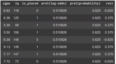
These residuals indicate how far off our initial model was from the actual label .

What We Do:

We now train a regression tree (not a classifier !) to predict the residuals.

• Input: cgpa, iq

• Target: Residuals r₁​

This regression tree becomes our first correction model :

                                               f₁(x)

Here’s the decision tree trained on residuals :

The tree learns to approximate the residuals based on the features—trying to minimize the squared error.

Why This Matters:

This is the heart of boosting. Instead of trying to get the correct answer directly, we build a model that learns how wrong we were, and use that to correct ourselves.

Each subsequent model will repeat this :

Predict residuals → Train regression tree → Add corrections

Step 2(c) : Calculating γ for Each Leaf Node (Part 1)

Once we've trained the regression tree, the next task is to calculate the output value for each leaf node, denoted by :

Hessian (Denominator)

Next, we need the second derivative :

Final Explanation in Words

• This gives the leaf output value γ for node 2.

• Similarly, we repeat the same computation for every leaf node in the regression tree.

• The computed γ for each node becomes the prediction/output that will be added to the ensemble model at the current boosting stage.

Step 2(d) : Updating the Model with the Tree Output

Now that we've trained our first regression tree on the residuals, it’s time to update our model.

Boosting Step – Model Update Rule

After fitting the regression tree to the residuals, we add its prediction to the current model’s output to improve it. This forms the basis of how boosting works :

                              f₁(x) = f₀(x) + output from decision tree

This updated model f₁(x) is now a better approximation of the true log-odds than f₀(x) , because it's been "boosted" by correcting its earlier mistakes .

Intuition

You’re not replacing the model. You’re stacking improvements .

Each tree tries to fix what the previous ensemble couldn’t .

Each step is a course correction, like GPS adjusting your route as you go off track .

That’s the essence of boosting: update → correct → repeat → converge .