
Support Vector Machine (SVM) – Part 4
- Aryan

- May 2, 2025
- 8 min read
Transition to SVM
This toy example builds the foundation for how SVM uses constrained optimization :
In SVM, we try to maximize the margin between two classes (analogous to maximizing z)
While ensuring all data points lie on the correct side of the margin (like satisfying the constraint x² + y² = 1)
The underlying geometry — finding the best solution on a constrained path — is exactly what makes SVMs powerful.
Understanding Gradient Vector Fields in the Context of Constrained Optimization
In the previous part, we saw how to maximize a function under a constraint using the geometric visualization of 3D surfaces and contour plots. Now we dive deeper into what the arrows in contour plots mean and how they help us find the optimum — this is where gradient vector fields come in.
What Does the New Plot Show ?
Let’s now examine a new graph :
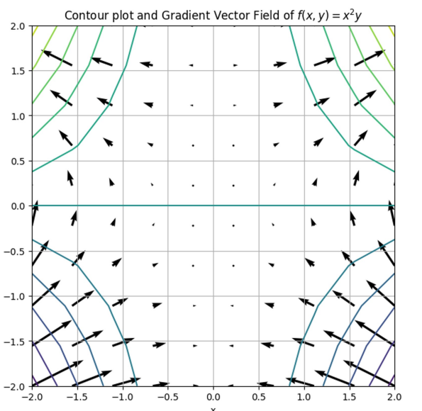
This plot includes :
Contour lines of the function — each line represents a set of (x,y) points where the function value (z) is constant.
Arrows that form the gradient vector field.
What Are These Arrows ?
These arrows represent the gradient of the function f(x, y) = x²y at different points.
The gradient of a multivariable function is a vector formed by the partial derivatives :
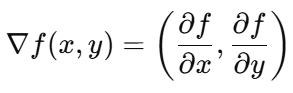
For our specific function f(x, y) = x²y , the gradient is :
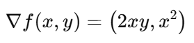
At every point (x , y), this gradient vector points in the direction in which f(x , y) increases the fastest — this is known as the direction of steepest ascent.
Gradient = Direction of Maximum Increase
Just like in single-variable calculus where the derivative tells you the slope of the function, in multivariable calculus the gradient tells you the slope and direction in which the function increases most rapidly.
The direction of the gradient vector points where z = f(x,y) increases fastest.
The length (magnitude) of the gradient vector tells how steep the increase is.
Gradient and Contour Lines : Orthogonality
There’s a beautiful geometric relationship between gradient vectors and contour lines :
The gradient vector at a point is always perpendicular to the contour line passing through that point.
Here’s why :
A contour line connects all points where the function has the same value (i.e., no change in z).
So, walking along a contour line means there is no change in function value.
But the gradient points in the direction where the function does change — the fastest.
Therefore, the direction of no change (contour) and the direction of maximum change (gradient) must be orthogonal.

Mathematical Summary of Gradient Properties
Let’s formalize this with key properties :
1. Direction of Maximum Change
The gradient ∇f points in the direction in which the function increases most rapidly.
2. Perpendicular to Contour Lines
If C is a contour line of f(x, y), and you are standing at a point on that line, the gradient vector will be perpendicular to the tangent vector of C at that point.
3. Magnitude = Steepness
If the gradient vector is long, the function is changing rapidly (contour lines are close).
If the gradient is small, the function is changing slowly (contour lines are far apart).
Intuition in Optimization
In optimization, understanding the gradient helps us :
Navigate the function surface.
Identify how to increase or decrease the function value.
Visualize constraints as boundaries within which the gradient must "push".
In our earlier constrained optimization problem, the solution occurred where the gradient of the function and the constraint interacted perfectly — geometrically, this is the point where the contour line of the objective function just touches the constraint curve, and the gradients of both are aligned.
Visual Takeaway
When we overlay :
Contour lines of a function,
And gradient vectors,
…we get a full geometric map of how the function behaves, where it increases most, and how constraints influence possible solutions.
This understanding of gradient behavior and constraints is exactly what underpins the mathematical foundation of SVMs, especially when we formulate them as a constrained optimization problem.
Gradient Alignment and Lagrange Multipliers — The Formal Condition for Constrained Optimization
We’ve seen how to visualize a function f(x,y) and a constraint like x² + y² = 1 using 3D plots, contours, and gradient fields. Now, we’ll take this one step further : how do we mathematically express the condition at the point where our function achieves its maximum (or minimum) under the constraint ?
Revisiting the Constraint
We’ve been working with a constraint :
x² + y² = 1
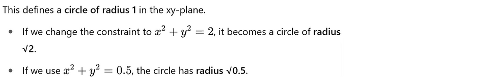
So, the constraint defines a family of circles.
Let’s now define this family more generally :
This defines a scalar field — for each point (x,y), it tells you how far you are from the origin squared.
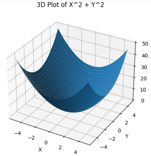
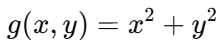
Contour Plot of g(x, y) = x² + y²
The contour lines of this function are concentric circles centered at the origin, each corresponding to a fixed value of g(x, y). These are just slices through the bowl.
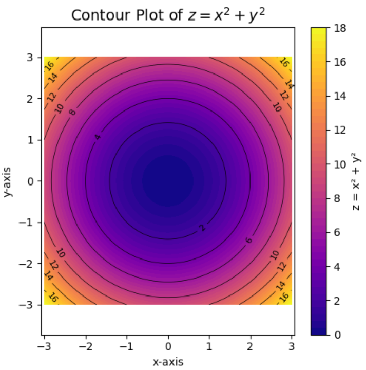
These circles represent level sets (points where the function has the same value), just like in topographic maps.
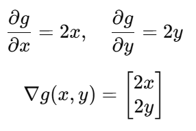
Gradient Vector Field of the Constraint Function
Because g(x, y) = x² + y² is a 3D surface, it too has a gradient vector field. For this function :
∇g(x,y) = (2x,2y)
These vectors point directly outward from the origin, perpendicular to each contour circle.

Notice that :
The vectors are perpendicular to the contour circles.
The farther from the origin, the larger the gradient vector.
The Key Insight : Tangency of Contour Lines

Each function has its own set of contour lines. Our task is to find the point where a contour line of f(x,y) just touches the constraint circle defined by g(x,y) = 1.

At this point of tangency :
Both contour lines touch at exactly one point.
Their gradients are perpendicular to their respective contour lines.
So, both gradients point in the same direction, even if their magnitudes differ.
Gradient Alignment = Lagrange Condition
This leads us to the mathematical condition for an optimum under constraint :

Here :
∇f(x,y) is the gradient of the function we are optimizing.
∇g(x,y) is the gradient of the constraint function.
λ (lambda) is a scalar multiplier, known as the Lagrange multiplier.
This equation says :
At the optimal point, the direction in which the function increases fastest (gradient of f) is exactly aligned with the direction in which the constraint changes (gradient of g).

Even if their magnitudes differ, they point along the same line, so one is a scalar multiple of the other.
Why This Matters
This condition — ∇f = λ∇g— is the core of Lagrange multipliers, a powerful method in optimization.
It lets us convert a constrained problem into a system of equations, which can be solved for the optimal point.
This is exactly what happens in Support Vector Machines :
SVMs optimize a function (maximize margin)
Subject to constraints (correct classification of data)
Using Lagrange multipliers to solve the problem
Final Summary of the Concept
Let’s wrap up this 3-part idea :
Optimization on a surface :
You want to maximize a function f(x, y) subject to a constraint g(x,y) = c.
Visualization :
The function’s surface is plotted in 3D.
The constraint is a curve (e.g., circle) lying on this surface.
The optimal point is where the surface is highest (or lowest) along the constraint.
Gradient and Contour Interplay :
Contours = level curves of constant value.
Gradients = point in direction of steepest ascent.
At the optimal point, the contours of f and g touch (are tangent).
So, their gradients are aligned : ∇f = λ∇g.
Transition to SVM
What we’ve built here is the full geometric and mathematical foundation for how SVMs perform optimization under constraints.
In the next step (outside these notes), we would define the specific SVM objective and constraints, then use Lagrange multipliers to derive the solution — just like we did here.
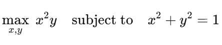
Using Lagrange Multipliers to Maximize f(x,y) = x²y
Subject to the constraint : x² + y² = 1
We are given :
Objective function : f(x,y) = x²y
Constraint : g(x,y) = x² + y² = 1
We use Lagrange multipliers, where the condition is :
∇f(x,y) = λ ∇g(x,y)
Here, λ is the Lagrange multiplier, and we compute gradients of f and g.
Step 1 : Compute the Gradients
Gradient of f(x,y) = x²y :

Gradient of g(x, y) = x² + y² :
Now applying the Lagrange condition :

This gives us two equations :
2xy = λ ⋅ 2x
x² = λ ⋅ 2y
Step 2 : Solve the Equations
From equation (1), assuming x ≠ 0, divide both sides by 2x :
y = λ ….(A)
Substitute (A) into equation (2):
x² = 2y² .…..(B)
Now substitute (B) into the constraint x² + y² = 1 :


Step 3 : Candidate Points
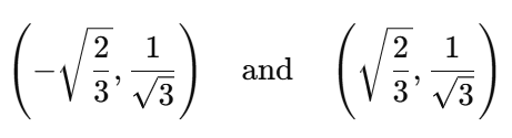
Possible values of (x,y) are :

Step 4 : Evaluate f (x,y) = x²y at These Points

Constraint Verification
Verify that each point satisfies x² + y² = 1 :

So all candidate points satisfy the constraint .
Visualization of the Lagrange Multiplier Solution
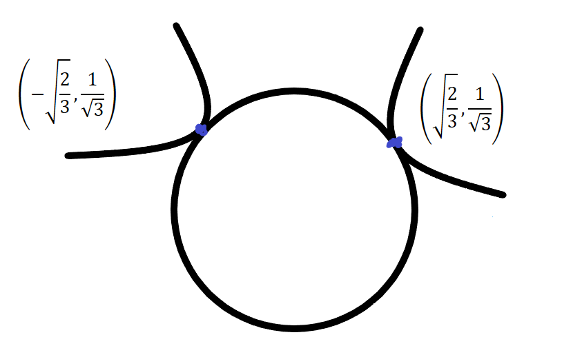
As we discussed earlier, there are two points that maximize the function f(x,y) = x²y under the constraint x² + y² = 1 :
This is the graphical representation of the solution. We’ve successfully solved a constrained optimization problem—we found the values of x and y that maximize z = f(x,y), while still satisfying the constraint x² + y² = 1 .
Why This Matters : Connecting to SVM
This simple example introduces the intuition behind solving constrained optimization problems, which is exactly what Support Vector Machines (SVM) require.
While our demo example involved maximizing a function subject to a geometric constraint (a circle), in SVM, the optimization problem is more complex and involves inequalities, slack variables, and regularization.
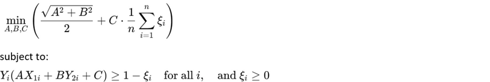
SVM Optimization Objective (Soft Margin SVM) :
We solve the following constrained optimization problem in soft-margin SVM :
Final Intuition :
The SVM optimization problem is far more difficult than our example—but solving the simpler case first helps build the intuition.
Just like our toy problem required gradients, constraints, and optimality conditions, SVM also uses these ideas—along with Lagrange multipliers and dual formulations—to find the optimal separating hyperplane.
Understanding this foundation gives us the conceptual clarity we need before diving into the technical derivation of SVM.
Understanding Lagrange Multipliers
Very useful in Support Vector Machines (SVM)
We are given a constrained optimization problem :

This is a problem where we want to maximize a function under a constraint.
Rewriting with Lagrange Multipliers
We can convert this constrained problem into a system of equations using Lagrange multipliers.
Let:
f(x, y) = x²y
g(x, y) = x² + y²
Then the condition becomes :
This gives us a system of equations whose solution gives us the maximum of f(x, y) on the constraint curve g(x,y) = 1 .
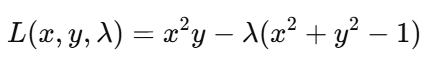
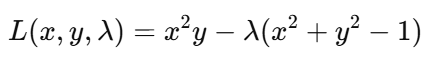
Alternate Formulation — Lagrangian Function
Another way to approach this is to turn the constrained problem into an unconstrained optimization problem by incorporating the constraint into the objective function using a multiplier λ.
We define the Lagrangian function :

That is :
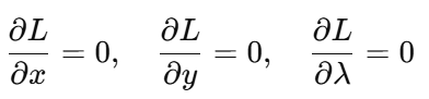
Now, to find the optimal solution, we solve :
This approach transforms a constrained problem into an unconstrained one, where the constraint becomes a part of the equation itself.
Why This Matters for SVM
This technique is foundational in SVM because we also transform a constrained optimization (maximize margin under classification constraints) into an unconstrained one using Lagrange multipliers—then solve it using calculus and duality.
How the Lagrangian Was Formed
Let’s now understand how the Lagrangian method works and why it gives us the same results as before.
Recap of Our Problem
We are solving :
We introduced the Lagrangian to turn this into an unconstrained problem :
To find the stationary points, we set the partial derivatives to zero :

Step-by-Step Derivation
1. Partial Derivative w.r.t. x :

2. Partial Derivative w.r.t. y :
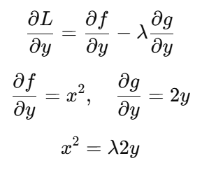
3. Partial Derivative w.r.t. λ :

This is just our original constraint.
Summary of the System
We now have a system of 3 equations :
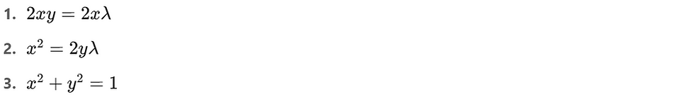
These are exactly the same equations we would have obtained using the gradient method :

Final Thoughts
We have discovered a second, powerful way to handle constrained optimization. Rather than solving the constraint separately, we:
Embed the constraint into the objective function using the Lagrangian.
Convert the constrained problem into a standard optimization problem.
Solve using calculus by setting partial derivatives to zero.
This approach is central to many optimization problems, especially in Support Vector Machines (SVMs) and machine learning in general.
